Cloud software, fragility and Air France 447

The Human Factor by William Langewiesche is an account of how Air France Flight 447 crashed back in 2009. It’s a great piece of long-form journalism.

[Recently deceased engineer Earl] Wiener pointed out that the effect of automation is to reduce the cockpit workload when the workload is low and to increase it when the workload is high.

That’s basically Nassim Nicholas Taleb’s definition of fragility: where the potential downside is much greater than the potential upside.

But this is what really struck me:

[U. Michigan Industrial & Systems Engineering Professor Nadine] Sarter said, “… Complexity means you have a large number of subcomponents and they interact in sometimes unexpected ways. Pilots don’t know, because they haven’t experienced the fringe conditions that are built into the system. I was once in a room with five engineers who had been involved in building a particular airplane, and I started asking, ‘Well, how does this or that work?’ And they could not agree on the answers. So I was thinking, If these five engineers cannot agree, the poor pilot, if he ever encounters that particular situation … well, good luck.””

We also build software by connecting together different subcomponents. We know that the hardware underlying these subcomponents can fail, and in order to provide reliability for our customers we must be able to deal with these failures. If we’re sophisticated, we turn to automation: we try to build fault-tolerant systems that can automatically detect failures and compensate for them.

But the behavior of these types of systems is difficult to reason about, precisely because they take action automatically based on self-monitoring. These systems can handle hard failures of individual components: when something has obviously failed. But if it’s a soft failure, where the component is still partially working, or if two independent components fail simultaneously, then the system may not be able to handle it. Adding automation to handle failures introduces new failure modes even as it eliminates old ones, and the new ones may be much harder for an operator to understand.

Consider the AWS outage of October 2012, which took down multiple websites that deploy on Amazon’s cloud. The outage was a result of:

1. A hardware failure on a data collection server
2. A DNS update not propagating to all internal DNS servers
3. A memory leak bug in an agent that monitors the health of EBS (storage) servers

The agents collect operational data from the storage servers and transfer it to data collection servers. Some agents couldn’t reach the collection servers because of a stale DNS entry. Because the agents also had a memory leak bug, they consumed too much memory on the storage servers.

Lack of sufficient memory is a good way to create a soft failure: the component still works, but in a degraded fashion. These memory-poor servers couldn’t keep up with requests, and eventually became stuck. The system detected the stuck servers (a hard failure), and failed over to healthy servers, but there were so many stuck servers that the healthy servers couldn’t keep up, and also became stuck.

The irony is that this failure is entirely due to the monitoring subsystem, which is intended to increase system reliability! It happened because of the co-incidence of a hardware failure in one component of the monitoring subsystem (a data collection server) and a software bug in another component of the monitoring subsystem (data collection agent).

We can’t avoid automation. In the case of the airlines, the automation has significantly increased safety, even though it increases the chances of incidents like Air France 447. For cloud software, this type of fault-tolerance automation does result in more reliable systems.

But, while these systems mean failure is less likely, when it does happen, it’s much more difficult to understand what’s happening. The future of cloud software is systems that fail much less often, but much harder. Buckle up.

Estimating confidence intervals, part 6

Our series of effort-estimation-in-the-small continues. This feature took a while to complete (where “complete” means “deployed to production”). I thought this was the longest feature I’d worked on, but looking at the historical data, there was another feature that took even longer.

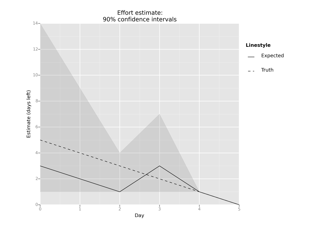
plot

Somehow, the legend has disappeared from the plot. The solid line is my best estimate of time remaining each day, and the dashed line is the true amount of time left. The grey area is my 90% confidence interval estimate.

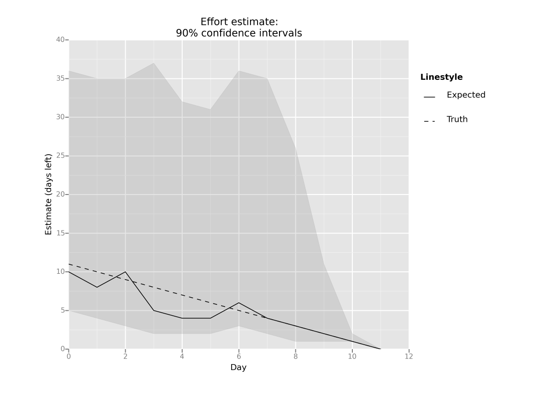
plot2

As usual, my “expected” estimate was much too optimistic. I initially estimated 10 days, where it actually took 17 days. I did stay within my 90% confidence interval, which gives me hope that I’m getting better at those intervals.

When I started this endeavor, my goal was to do a from-scratch estimate each day, but that proved to require too much mental effort, and I succumbed to the anchoring effect. Typically, I would just make an adjustment to the previous day’s estimate.

Interestingly, when I was asked in meetings how much time was left to complete this feature, I gave off-the-cuff (and, unsurprisingly, optimistic) answers instead of consulting my recorded estimates and giving the 90% interval.

Good to great

A few months ago I read Good to Great, a book about the factors that led to companies making a transition from being “good” to being “great”. Collins, the author, defines “great” as companies whose stock performed at least three times better than the overall market over at least fifteen years. While the book is ostensibly about a  research study, it feels packaged as a set of recommendations for executives looking to turn their good companies into great ones.

The lessons in the book sound reasonable, but here’s the thing: If Collins’s theory is correct, we should be able to identify companies that will outperform the market by a factor of three in fifteen-years time, by surveying employees to see if they meet the seven criteria outlined in the book.

It has now been almost thirteen years since the book has been published. Where are the “Good to Great” funds?

Estimating confidence intervals, part 4

Here’s the latest installment in my continuing saga to estimate effort with 90% confidence intervals. Here’s the plot:

plot

In this case, my estimate of the expected time to completion was fairly close to the actual time. The upper end of the 90% confidence interval is extremely high, largely because there was some work that I considered optional to complete the feature that decided to put off to some future data.

Here’s the plot of the error:

plot2It takes a non-trivial amount of mental efforts to do these estimates each day. I may stop doing these soon.


Not apprenticeship!

Mark Guzdial points to an article by Nicholas Lemann in the Chronicle of Higher Ed entitled The Soul of the Research University. It’s a good essay about the schizophrenic nature of the modern research university. But Lemann takes some shots at the notion of teaching skills in the university. Here’s some devil’s advocacy from the piece:

Why would you want to be taught by professors who devote a substantial part of their time to writing projects, instead of working professionals whose only role at the university is to teach? Why shouldn’t the curriculum be devoted to imparting the most up-to-the-minute skills, the ones that will have most value in the employment market? Embedded in those questions is a view that a high-quality apprenticeship under an attentive mentor would represent no loss, and possibly an improvement, over a university education.

Later on, Lemann refutes that perspective, that students are better off being taught at research universities by professors engaged in research. He seems to miss the irony that this apprenticeship model is precisely how these research universities train PhD students. For bonus irony, here was the banner ad I saw atop the article: skills-webinar

Estimating confidence intervals, part 3

Another episode in our continuing series of effort estimation in the small with 90% confidence intervals. I recently finished implementing another feature after doing the effort estimates for each day. Here’s the plot:


Effort estimation, 90% confidence intervals

Once again, I underestimated the effort even at the 90% level, although not as badly as last time. Here’s a plot of the error.

Error plot

I also find it takes real mental energy to do these daily effort estimates.


Crossing the river with TLA+

Lately, I’ve been interested in approaches to software specifications that are amenable to model checking. A few weeks ago in this blog, I wrote about solving a logic puzzle with Alloy. Today’s post is about solving a different logic puzzle. I found this one from the Alloy online tutorial:

A farmer is on one shore of a river and has with him a fox, a chicken,
and a sack of grain. He has a boat that fits one object besides himself.

In the presence of the farmer nothing gets eaten, but if left without the
farmer, the fox will eat the chicken, and the chicken will eat the grain.
How can the farmer get all three possessions across the river safely?

To solve this, I used TLA+, a specification language developed by Leslie Lamport. It also uses PlusCal, which is an algorithm language that can be automated translated into TLA+ using the TLA toolbox.

Here’s my solution, which includes PlusCal but doesn’t show the automatically translated parts of the model.

-------------------------------- MODULE boat --------------------------------
EXTENDS Integers, FiniteSets
CONSTANTS Farmer, Fox, Chicken, Grain
CREATURES == {Farmer, Fox, Chicken, Grain}

alone(animals, side) == (animals \in SUBSET side) /\ ~ Farmer \in side

somebodyGetsEaten(l, r) == \/ alone({Fox, Chicken}, l)
                           \/ alone({Fox, Chicken}, r)
                           \/ alone({Chicken, Grain}, l)
                           \/ alone({Chicken, Grain}, r)

safe(l, r) == ~somebodyGetsEaten(l, r)

safeBoats(from, to) ==
    { boat \in SUBSET from : /\ Farmer \in boat
                             /\ Cardinality(boat) <= 2
                             /\ safe(from \ boat, to \cup boat) }   
(***************************************************************************
    --algorithm RiverCrossing {
    variables left = CREATURES; right = {};
    process ( LeftToRight = 0 )
        { l: while (left /= {})
             { await (Farmer \in left);
               with(boat \in safeBoats(left, right))
                 {
                   left := left \ boat;
                   right := right \cup boat
                 }
             }
        }
    process ( RightToLeft = 1 )
        { r: while (left /= {})
             { await (Farmer \in right);
               with(boat \in safeBoats(right, left))
                 {
                   left := left \cup boat;
                   right := right \ boat
                 }
             }
        }
    }
***************************************************************************)

============================================================

To solve the problem with the TLA toolbox, you’ll need to specify an invariant that will be violated when the puzzle is solved. I used right /= CREATURES.

Run the model, and it will produce a trace that violates the invariant:


error-trace

(You’ll first need to translate the PlusCal into TLA+, and you’ll need to specify the value of the constants. I just chose “Model value” for each of them).

You can see the full model with the automatic PlusCal translation in one of my Github repos.

Estimating confidence intervals, part 2

Here is another data point from my attempt to estimate 90% confidence intervals. This plot shows my daily estimates for completing a feature I was working on.

90% confidence intervals


The dashed line is the “truth”: it’s what my estimate would have been if I had estimated perfectly each day. The shaded region represents my 90% confidence estimate: I was 90% confident that the amount of time left fell into that region. The solid line is the traditional pointwise effort estimate: it was my best guess as to how many days I had left before the feature would be complete.

For this feature, I significantly underestimated the effort required to complete it. For the first four days, my estimates were so off that my 90% confidence interval didn’t include the true completion time: it was only correct 60% of the time.

This plot shows the error in my estimates for each day:


Error in effort estimate

Apparently, I’m not yet a well-calibrated estimator. Hopefully, that will improve with further estimates.

Presentation as text

I gave a talk last week at Camp DevOps about Ansible and EC2. The talk is written in present format, which is a very lightly marked up text format, similar to Markdown. You can see the source file in a Github repo.

It was liberating to focus entirely on content and not worry too much about the exact appearance of the slide.

I also went for a minimalistic approach where I often didn’t even use titles. The slides won’t make much sense if you just look at them without me talking. Hopefully, they made some sense when I was talking in front of them.