The Tortoise and the Hare in Alloy

If you’ve done your share of leetcode-style interviewing, and you’re above a certain age, you may have been asked during a technical screen to write a program that determines if a linked list contains a cycle. If the interviewer was really tough on you, they might have asked how to implement this in O(1) space.

There’s a well-known O(1) algorithm for finding cycles in linked lists, attributed to Robert Floyd, called the tortoise and the hare. I’ve previously written about modeling this algorithm in TLA+. In this post, I’m going to do it in Alloy. Version 6 of Alloy added support for temporal operators, which makes it easier to write TLA+ style models, with the added benefit of Alloy’s visualizer. This was really just an excuse for me to play with these operators.

You can find my model at https://github.com/lorin/tortoise-hare-alloy/

Brief overview of the algorithm

Basic strategy: define two pointers that both start at the head of the list. At each iteration, you advance one of the pointers (the tortoise) by one step, and the other (the hare) by two steps. If the hare reaches the tail of the list, there are no cycles. If the tortoise and the hare ever point to the same node, there’s a cycle.

With that out of the way, let’s model this algorithm in Alloy!

Linked lists

Let’s start off by modeling linked lists. Here’s the basic signature.

sig Node {
    next : lone Node
}

Every linked list has a head. Depending on whether there’s a cycle, it may or may not have a tail. But we do know that it has at most one tail.

one sig Head in Node {}
lone sig Tail in Node {}

Let’s add a fact about the head, using Alloy reflexive transitive closure operator (*).

fact "all nodes are reachable from the head" {
    Node in Head.*next
}

You can think of Head.*next as meaning “every node that is reachable from Head, including Head itself”.

Finally, we’ll add a fact about the tail:

fact "the tail is the only node without a successor" {
    all n : Node | no n.next <=> n = Tail
}

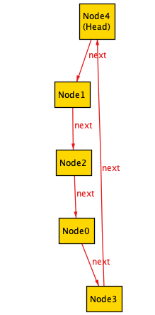
We can now use Alloy to generate some instances for us to look at. Here’s how to tell Alloy to generate an instance of the model that contains 5 nodes and has a tail:

acyclic: run { some Tail } for exactly 5 Node

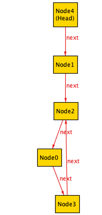
This is what we see in the visualizer:

We can also tell Alloy to generate an instance without a tail:

cycle: run { no Tail } for exactly 5 Node

Here are three different instances without tails:
Tortoise and hare tokens

The tortoise and the hare are pointers to the nodes. However, I like to think of them like tokens moving along a game board, so I called them tokens. Here’s how I modeled them:

abstract sig Token {
    var at : Node
}

one sig Tortoise, Hare extends Token {}

Note that the Token.at field has a var prefix. That’s new in Alloy 6, and it means that the field can change over time.

As in TLA+, we need to specify the initial state for variables that change over time. Both tokens start at the head, which we can express as a fact.

fact init {
    Token.at in Head
}

Next, as in TLA+, we need to model how variables change over time.

Here’s the predicate that’s true whenever the tortoise and hare take a step. Alloy uses the same primed variable notation as TLA+ to refer to “the value of the variable in the next state”. In TLA+, we’d call this kind of predicate an action, because it contains primed variables:

pred move {
    Tortoise.at' = advance[Tortoise.at]
    Hare.at' = advance[advance[Hare.at]]
}

This predicate uses a helper function I wrote called advance which takes a pointer to a node and advances to the next node, unless it’s at the tail, in which case it stays where it is:

fun advance[n : Node] : Node {
    (n = Tail) implies n else n.next
}

We can run our model like this, using the always temporal operator to indicate that the move predicate is true at every step.

run {always move} for exactly 5 Node

Here’s a screenshot of Alloy’s visualizer UI for one of the traces. You can see that there are 5 states in the trace, and it’s currently displaying state 2.

Here are all of the states in the trace:
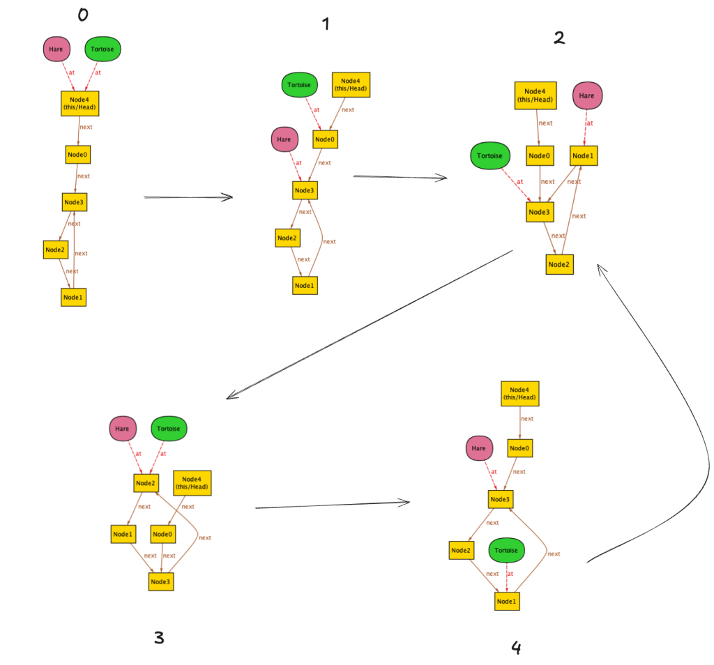
It’s confusing to follow what’s happening over time because Alloy re-arranges the layout of the nodes at the different steps. We’ll see later on this post how we can configure the visualizer so to make it easier to follow.

Output of the algorithm

So far we’ve modeled the movement of the tortoise and hare tokens, but we haven’t fully modeled the algorithm, because we haven’t modeled the return value, which is supposed to indicate whether there’s a cycle or not.

I modeled the return value as a Result signature, like this:

abstract sig CycleStatus {}
one sig Cycle, NoCycle, Running extends CycleStatus {}

var one sig Result in CycleStatus {}

You can think of Result as being like an enum, which can take on values of either Cycle, NoCycle, or Running.

Note that Result has a var in front, meaning it’s a variable that can change over time. It starts off in the Running state, so let’s augment our init fact:

fact init {
    Token.at in Head
    Result = Running
}

Let’s also define termination for this algorithm. Our algorithm is done when Result is either Cycle or NoCycle. Once it’s done, we no longer need to advance the tortoise and hare pointers. We also don’t change the result once the program has terminated.

pred done {
    Result in Cycle + NoCycle
    Tortoise.at' = Tortoise.at
    Hare.at' = Hare.at
    Result' = Result
}

We need to update the move action so that it updates our Result variable. We also don’t want the move action to be enabled when the algorithm is done (no need to keep advancing the pointers), so we’ll add an enabling condition. As a result, move now looks like this:

pred move {
  // enabling condition
  Result = Running

  // advance the pointers
  Tortoise.at' = advance[Tortoise.at]
  Hare.at' = advance[advance[Hare.at]]

  // update Result if the hare has reached the tail 
  // or tortoise and hare are at the same node
  Hare.at' = Tail implies Result' = NoCycle
                  else    Hare.at' = Tortoise.at' implies Result' = Cycle
                                                  else    Result' = Result
}

The syntax for updating the Result isn’t as nice as in TLA+: Alloy doesn’t have a case statement. It doesn’t even have an if statement: instead we use implies/else to achieve if/else behavior.

We can now define the full spec like this:

pred spec {
    always (
        move or
        done
    )
}

And then we can ask the analyzer to generate traces when spec is true, like this:

example: run { spec } for exactly 5 Node

Improving the visualization

Finally, let’s make the visualization nicer to look at. I didn’t want the tortoise and hare to be rendered by the visualizer as objects separate from the nodes. Instead I wanted them to be annotations on the node.

The analyzer will let you represent fields as attributes, so I could modify the Node signature to add a new field that contains which tokens are currently occupying the node:

sig Node {
    next : lone Node,
    var tokens : set Token // <- new field (I didn't do this)
}

But I didn’t want to add a field to my model.

However, Alloy lets you define a function that returns a Node -> Token relation, and then the visualizer will let you treat this function like it’s a field. This relation is just the inverse of the at relationship that we defined on the Token signature:

// This is so the visualizer can show the tokens as attributes 
// on the nodes
fun tokens[] : Node -> Token {
    ~at
}

Now, in the theme panel of the visualizer, there’s a relation named $tokens.

You can also rename things. In particular, I renamed Tortoise to 🐢 and Hare to 🐇 as well as making them attributes. Here’s a screenshot after the changes:

Here’s an example trace when there’s no cycle. Note how the (Result) changes from Running to NoCycle

Much nicer!

Checking a property

Does our program always terminate? We can check like this:

assert terminates {
    spec => eventually done
}

check terminates for  exactly 5 Node

The analyzer output looks like this:

Solving...
No counterexample found. Assertion may be valid. 9ms.

In general, this sort of check doesn’t guarantee that our program terminates, because our model might be too small.

We can also check for correctness. Here’s how we can ask Alloy to check that there is a cycle in the list if and only if the program eventually terminates with Result=Cycle.

pred has_cycle {
    some n : Node | n in n.^next
}

assert correctness {
     spec => (has_cycle <=> eventually Result=Cycle)
}

check correctness for exactly 5 Node

Note that we’re using the transitive closure (^) in the has_cycle predicate to check if there’s a cycle. That predicate says: “there is some node in that is reachable from itself”.

Further reading

For more on Alloy 6, check out the following:

Alloy’s very easy to get started with: I recommend you give it a go!
Reading the Generalized Isolation Level Definitions paper with Alloy

My last few blog posts have been about how I used TLA+ to gain a better understanding of database transaction consistency models. This post will be in the same spirit, but I’ll be using a different modeling tool: Alloy.

Like TLA+, Alloy is a modeling language based on first-order logic. However, Alloy’s syntax is quite different: defining entities in Alloy feels like defining classes in an object-oriented language, including the ability to define subtypes. It has first class support for relations, which makes it very easy to do database-style joins. It also has a very nifty visualization tool, which can help when incrementally defining a model.

I’m going to demonstrate here how to use it to model and visualize database transaction execution histories, based on the paper Generalized Isolation Level Definitions by Atul Adya, Barbara Liskov and Patrick O’Neil. This is a shorter version of Adya’s dissertation work, which is referenced frequently on the Jepsen consistency models pages.

There’s too much detail in the models to cover in this blog post, so I’m just going to touch on some topics. If you’re interested in more details, all of my models are in my https://github.com/lorin/transactions-alloy repository.

Modeling entities in Alloy

Let’s start with a model with the following entiteis:

  • objects
  • transactions (which can commit or abort)
  • events (read, write, commit, abort)

The diagram below shows some of the different entities in our Alloy model of the paper.

You can think of the above like a class diagram, with the arrows indicating parent classes.

Objects and transactions

Objects and transactions are very simple in our model.

sig Object {}

abstract sig Transaction {}

sig AbortedTransaction, CommittedTransaction extends Transaction {}

The word sig is a keyword in Alloy that means signature. Above I’ve defined transactions as abstract, which means that they can only be concretely instantiated by subtypes.

I have two subtypes, one for aborted transactions, one for committed transactions.

Events

Here are the signatures for the different events:

abstract sig Event {
    tr: Transaction,
    eo: set Event, // event order (partial ordering of events)
    tnext: lone Event // next event in the transaction
}

// Last event in a transaction
abstract sig FinalEvent extends Event {}

sig Commit extends FinalEvent {}

sig Abort extends FinalEvent {}

sig Write extends Event {
    obj: Object,
    wn : WriteNumber
}

sig Read extends Event {
    sees: Write // operation that did the write
}

The Event signature has three fields:

  • tr – the transaction associated with the event
  • eo – an event ordering relationship on events
  • tnext – the next event in the transaction

Reads and writes each have additional fielsd.

Reads

A read has one custom field, sees. In our model, a read operation “sees” a specific write operation. We can follow that relationship to identify the object and the value being written.

Writes and write numbers

The Write event signature has two additional fields:

  • obj – the object being written
  • wn – the write number

Following Adya, we model the value of a write by a (transaction, write number) pair. Every time we write an object, we increment the write number. For example, if there are multiple writes to object X, the first write has write number 1, the second has write number 2, and so on.

We could model WriteNumber entities as numbers, but we don’t need full-fledged numbers for this behavior. We just need an entity that has an order defined (e.g., it has to have a “first” element, and each element has to have a “next” element). We can use the ordering module to specify an ordering on WriteNumber:

open util/ordering[WriteNumber] as wo

sig WriteNumber {}

Visualizing

We can use the Alloy visualizer to generate a visualization of our model. To do that, we just need to use the run command. Here’s the simplest way to invoke that command:

run {} 

Here’s what the generated output looks like:

Visualization of a history with the default theme

Yipe, that’s messy! We can clean this up a lot by configuring the theme in the visualizer. Here’s the same graph, with different theme settings. I renamed several things (e.g., “Ta” instead of “AbortedTransaction”), I had some relationships I didn’t care about (eo), and I showed some relationships as attributes instead of arcs (e.g., tr).

Visualization after customizing the theme

The diagram above shows two transactions (Ta, Tc). Transaction Ta has a read operation (Read) and a write operation (Write0). Transaction Tc has a write operation. (Write1).

Constraining the model with facts

The history above doesn’t make much sense:

  • tnext is supposed to represent “next event in the transaction”, but in each transaction, tnext has loops in it
  • Ta belongs to the set of aborted transactions, but it doesn’t have an abort event
  • Tc belongs to the set of committed transactions, but it doesn’t have a commit event

We need to add constraints to our model so that it doesn’t generate nonsensical histories. We do this in Alloy by adding facts.

For example, here are some facts:

// helper function that returns set of events associated with a transaction
fun events[t : Transaction] : set Event {
    tr.t
}

fact "all transactions contain exactly one final event" {
    all t : Transaction | one events[t] & FinalEvent
}

fact "nothing comes after a final event" {
    no FinalEvent.tnext
}

fact "committed transactions contain a commit" {
    all t : CommittedTransaction | some Commit & events[t]
}

fact "aborted transactions contain an abort" {
    all t : AbortedTransaction | some Abort & events[t]
}

Now our committed transactions will always have a commit! However, the facts above aren’t sufficient, as this visualization shows:

I won’t repeat all of the facts here, you can see them in the transactions.als file.

Here’s one last example of a fact, encoded from the Adya paper:

The corresponding fact in my model is:

/**
 * If an event wi (xi:m) is followed by ri (xj) without an intervening event wi (xi:n) in E, xj must be xi:m
 */
fact "transaction must read its own writes" {
    all T : Transaction, w : T.events & Write, r : T.events & Read | ({
            w.obj = r.sees.obj
            w->r in eo
            no v : T.events & Write | v.obj = r.sees.obj and (w->v + v->r) in eo
    } => r.sees = w)
}

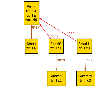
With the facts specified, our generated histories no longer look absurd. Here’s an example:

Mind you, this still looks like an incorrect history: we have two transactions (Tc1, Tc0) that commit after reading a write from an aborted transaction (Ta).

Installed versions

The paper introduces the concept of a version of an object. A version is installed by a committed transaction that contains a write.

I modeled versions like this.

open util/ordering[VersionNumber] as vo

sig VersionNumber {}

// installed (committed) versions
sig Version {
    obj: Object,
    tr: one CommittedTransaction,
    vn: VersionNumber
}

Dependencies

Once we have versions defined, we can model the dependencies that Adya defines in his paper. For example, here’s how I defined the directly write-depends relationship, which Adya calls ww in his diagrams.

fun ww[] : CommittedTransaction -> CommittedTransaction {
    { disj Ti, Tj : CommittedTransaction | some v1 : installs[Ti], v2 : installs[Tj] | {
        same_object[v1, v2]
        v1.tr = Ti
        v2.tr = Tj
        next_version[v1] = v2
        }
    }
}

Visualizing counterexamples

Here’s a final visualizing example of visualizations. The paper A Critique of ANSI SQL Isolation Levels by Berenson et al. provides some formal definition of different interpretations of the ANSI SQL specification. One of them they call “anomaly serializable (strict interpretation)”.

We can build a model this interpretation in Alloy. Here’s part of it just to give you a sense of what it looks like, see my bbg.als file for the complete model:

pred AnomalySerializableStrict {
    not A1
    not A2
    not A3
}

/**
 * A1: w1[x]...r2[x]...(a1 and c2 in any order)
 */
pred A1 {
    some T1 : AbortedTransaction,
         T2 : CommittedTransaction,
         w1: Write & events[T1],
         r2 : Read & events[T2],
         a1 : Abort & events[T1] | {

       w1->r2 in teo
       r2.sees = w1
       // r2 has to happen before T1 aborts
       r2->a1 in teo
    }
}

...

And then we can ask Alloy to check whether AnomalySerializableStrict implies Adya’s definition of serializability (which he calls isolation level PL-3).

Here’s how I asked Alloy to check this:

assert anomaly_serializable_strict_implies_PL3 {
    always_read_most_recent_write => (b/AnomalySerializableStrict => PL3)
}

check anomaly_serializable_strict_implies_PL3
for 8 but exactly 3 Transaction, exactly 2 Object, exactly 1 PredicateRead, exactly 1 Predicate

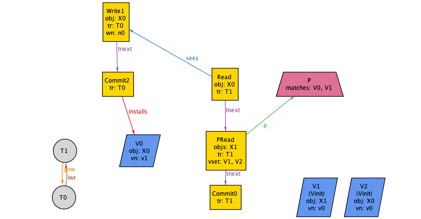
Alloy tells me that the assertion is invalid, and shows the following counterexample:

This shows a history that satisfies the anomaly serializable (strict) specificaiton, but not Adya’s PL-3. Note that the Alloy visualizer has generated a direct serialization graph (DSG) in the bottom left-hand corner, which contains a cycle.

Predicate reads

This counterexample involves predicate reads, which I hadn’t shown modeled before, but they look like this:

// transactions.als

abstract sig Predicate {}

abstract sig PredicateRead extends Event {
    p : Predicate,
    objs : set Object
}

// adya.als

sig VsetPredicateRead extends PredicateRead {
    vset : set Version
}

sig VsetPredicate extends Predicate {
    matches : set Version
}

A predicate read is a read that returns a set of objects.

In Adya’s model, a predicate read takes as input a version set (a version for each object) and then determines which objects should be included in the read based on whether or not the versions match the predicate:

fact "objects in predicate read are the objects that match in the version set" {
    all pread : VsetPredicateRead |
        pread.objs = (pread.vset & pread.p.matches).obj
}

One more counterexample

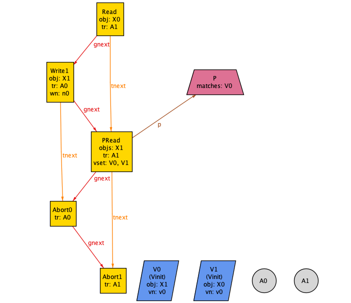
We can also use Alloy to show us when a transaction would be permitted by Adya’s PL-3, but forbidden by the broad interpretation of anomaly serializability:

check PL3_implies_anomaly_serializable_broad
for 8 but exactly 3 Transaction, exactly 2 Object, exactly 1 PredicateRead, exactly 1 Predicate

assert PL3_implies_anomaly_serializable_broad {
    always_read_most_recent_write => (PL3 => b/AnomalySerializableBroad)
}

The example above shows the “gnext” relation, which yields a total order across events.

The resulting counterexample is two aborted transactions! Those are trivially serializable, but it is ruled out by the broad definition, specifically, P3:

Playing with Alloy

I encourage you to try Alloy out. There’s a great Visual Studio code plugin that will let you execute your Alloy models from VS Code, that’s what I’ve been using. It’s very easy to get started with Alloy, because you can get it to generate visualizations for you out of the simplest models.

For more resources, Hillel Wayne has written a set of Alloy docs that I often turn to. There’s even an entire book on Alloy written by its creator. (Confusingly, though, the book does not have the word Alloy in the name).