Back in August, Murat Derimbas published a blog post about the paper by Herlihy and Wing that first introduced the concept of linearizability. When we move from sequential programs to concurrent ones, we need to extend our concept of what “correct” means to account for the fact that operations from different threads can overlap in time. Linearizability is the strongest consistency model for single-object systems, which means that it’s the one that aligns closest to our intuitions. Other models are weaker and, hence, will permit anomalies that violate human intuition about how systems should behave.
Beyond introducing linearizability, one of the things that Herlihy and Wing do in this paper is provide an implementation of a linearizable queue whose correctness cannot be demonstrated using an approach known as refinement mapping. At the time the paper was published, it was believed that it was always possible to use refinement mapping to prove that one specification implemented another, and this paper motivated Leslie Lamport and Martín Abadi to propose the concept of prophecy variables.
I have long been fascinated by the concept of prophecy variables, but when I learned about them, I still couldn’t figure out how to use them to prove that the queue implementation in the Herlihy and Wing paper is linearizable. (I even asked Leslie Lamport about it at the 2021 TLA+ conference).
Recently, Lamport published a book called The Science of Concurrent Programs that describes in detail how to use prophecy variables to do the refinement mapping for the queue in the Herlihy and Wing paper. Because the best way to learn something is to explain it, I wanted to write a blog post about this.
In this post, I’m going to assume that readers have no prior knowledge about TLA+ or linearizability. What I want to do here is provide the reader with some intuition about the important concepts, enough to interest people to read further. There’s a lot of conceptual ground to cover: to understand prophecy variables and why they’re needed for the queue implementation in the Herlihy and Wing paper requires an understanding of refinement mapping. Understanding refinement mapping requires understanding the state-machine model that TLA+ uses for modeling programs and systems. We’ll also need to cover what linearizability actually is.
We’ll going to start all of the way at the beginning: describing what it is that a program should do.
What does it mean for a program to be correct?
Think of an abstract data type (ADT) such as a stack, queue, or map. Each ADT defines a set of operations. For a stack, it’s push and pop , for a queue, it’s enqueue and dequeue, and for a map, it’s get, set, and delete.
Let’s focus on the queue, which will be a running example throughout this blog post, and is the ADT that is the primary example in the linearizability paper. Informally, we can say that dequeue returns the oldest enqueued value that has not been dequeued yet. It’s sometimes called a “FIFO” because it exhibits first-in-first-out behavior. But how do we describe this formally?
Think about how we would test that a given queue implementation behaves the way we expect. One approach is write a test that consists of a history of enqueue and dequeue operations, and check if our queue returns the expected values.
Here’s an example of an execution history, where enq is the enqueue operation and deq is the dequeue operation. Here I assume that enq does not return a value.
enq("A")
enq("B")
deq() → "A"
enq("C")
deq() → "B"
deq() → "C"
If we have a queue implementation, we can make these calls against our implementation and check that, at each step in the history, the operation returns the expected value, something like this:
Queue q = new Queue();
q.enq("A");
q.enq("B");
assertEquals("A", q.deq());
q.enq("C");
assertEquals("B", q.deq());
assertEquals("C", q.deq());
Of course, a single execution history is not sufficient to determine the correctness of our queue implementation. But we can describe the set of every possible valid execution history for a queue. The size of this set is infinite, so we can’t explicitly specify each history like we did above. But we can come up with a mathematical description of the set of every possible valid execution history, even though it’s an infinite set.
Specifying valid execution histories: the transition-axiom method
In order to specify how our system should behave, we need a way of describing all of its valid execution histories. We are particularly interested in a specification approach that works for concurrent and distributed systems, since those systems have historically proven to be notoriously difficult for humans to reason about.
In the 1980s, Leslie Lamport introduced a specification approach that he called the transition-axiom method. He later designed TLA+ as a language to support specifying systems using the transition-axiom method.
The transition-axiom method uses a state-machine model to describe a system. You describe a system by describing:
- The set of valid initial states
- The set of valid state transitions
(Aside: I’m not covering the more advanced topic of liveness in this post).
A set of related state transitions is referred to as an action. We use actions in TLA+ to model the events we care about (e.g., calling a function, sending a message).
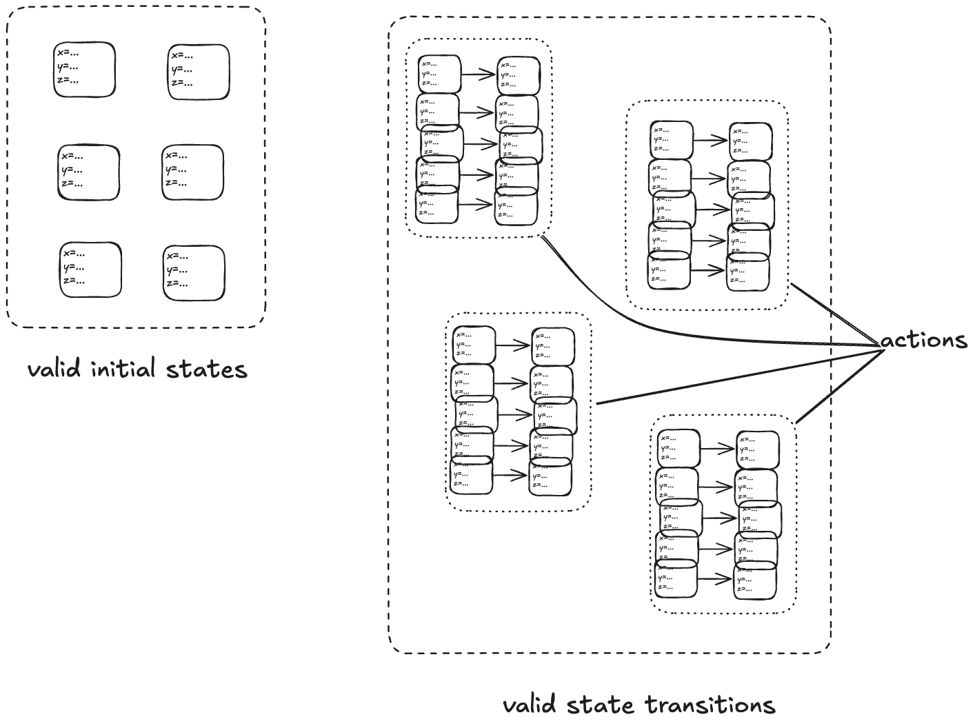
With a state-machine description, we can generate all sequences that start at one of the initial states and transition according to the allowed transitions. A sequence of states is called a behavior. A pair of successive states is called a step.
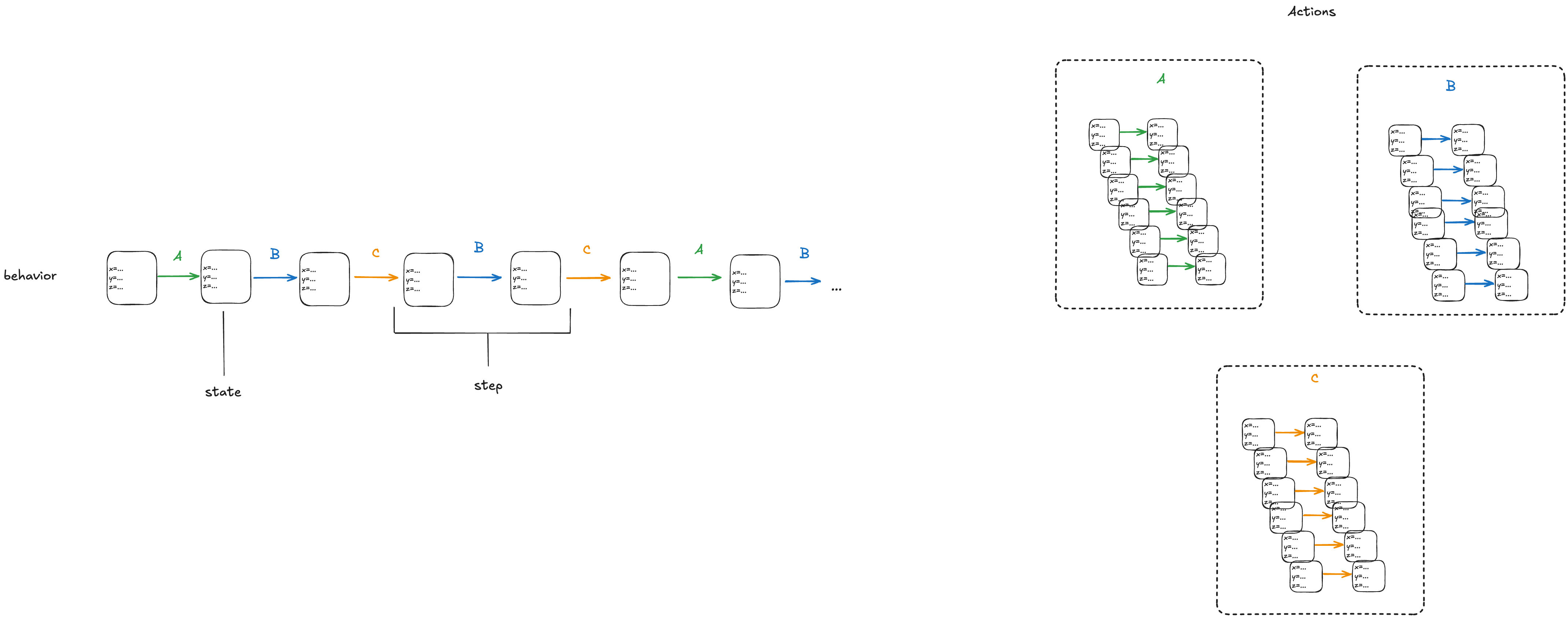
Each step in a behavior must be a member of one of the actions. In the diagram above, we would call the first step an A-step because it is a step that is a member of the A action.
We refer to the set that includes all of the actions as the next-state action, which is typically called Next in TLA+ specifications.
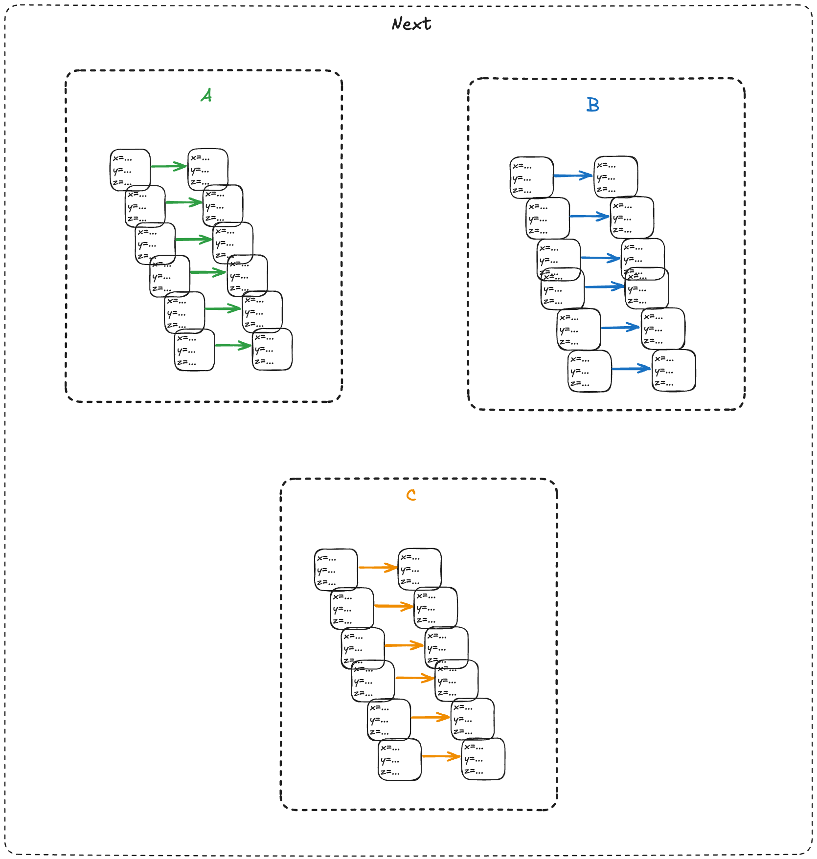
In the example above, we would say that A, B, C are sub-actions of the Next action.
We call the entire state-machine description a specification: it defines the set of all allowed behaviors.
To make things concrete, let’s start with a simple example: a counter.

Modeling a counter with TLA+
Consider a counter abstract data type, that has only two operations:
- inc – increment the counter
- get – return the current value of the counter
- reset – return the value of the counter to zero
Here’s an example execution history.
inc()
inc()
get() → 2
get() → 2
reset()
get() → 0
To model this counter in TLA+, we need to model the different operation types (inc, get, reset). We also need to model the return value for the get operation. I’ll model the operation with a state variable named op, and the return value with a state variable named rval.
But there’s one more thing we need to add to our model. In a state-machine model, we model an operation using one or more state transitions (steps) where at least one variable in the state changes. This is because all TLA+ models must allow what are called stuttering steps, where you have a state transition where none of the variables change.
This means we need to distinguish between two consecutive inc operations versus an inc operation followed by a stuttering step where nothing happens.
To do that, I’ll add a third variable to my model, which I’ll unimaginatively call flag. It’s a boolean variable, which I will toggle every time an operation happens. To sum up, my three state variables are:
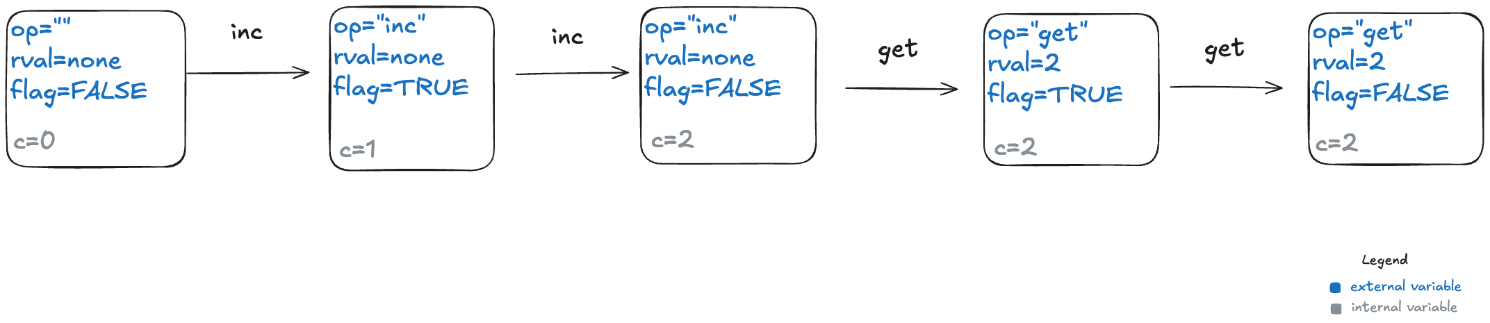
- op – the operation (“inc”, “get”, “reset”), which I’ll initialize to “” (empty string) in the first state
- rval – the return value for a get operation. It will be a special value called none for all of the other operations
- flag – a boolean that toggles on every (non-stuttering) state transition.
Below is a depiction of an execution history and how this would be modeled as a behavior at TLA+. The text in red indicated which variable changed in the transition. As mentioned above, every transition associated with an operation must have at least one variable that changes value.
Here’s a visual depiction of an execution history. Note how each event in the history is modeled as a step (pair of states) where at least one variable changes.

To illustrate why we need the extra variables, consider the following three behaviors.
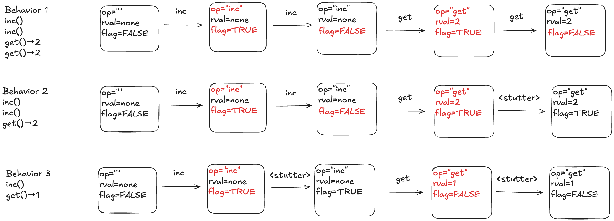
In behavior 1, there are no stuttering steps. In behavior 2, the last step is a stuttering step, so there is only one “get” invocation. In behavior 3, there are two stuttering steps.
The internal variables
Our model of a counter so far has defined the external variables, which are the only variables that we really care about as the consumer of a specification. If you gave me a set of all of the valid behaviors for a queue, where behaviors were described using only these external behaviors, that’s all I need to understand how a queue behaves.
However, the external variables aren’t sufficient for the producer of a specification to actually generate the set of valid behaviors. This is because we need to keep track of some additional state information: how many increments there have been since the last reset. This type of variable is known as an internal state variable. I’m going to call this particular internal state variable c.
Here’s behavior 1, with different color codings for the external and internal variables.
The actions
Here is a visual depiction of the permitted state transitions. Recall the set of permitted state transitions is called an action. For our counter, there are three actions, which corresponds to the three different operations we model: inc, get, and reset.
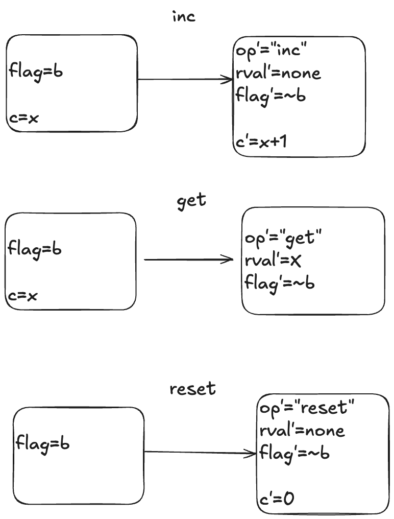
Each transition is depicted as two boxes with variables in it. The left-hand box shows the values of the variables before the state transition, and the right-hand box shows the values of the variables after the state transition. By convention we add a prime (‘) to the variables to refer to their values after the state transition.
While the diagram depicts three actions, each action describes a set of allowed state transitions. As an example, here are two different state transitions that are both members of the inc set of permitted transitions.
- [flag=TRUE, c=5] → [flag=FALSE, c=6]
- [flag=TRUE, c=8]→ [flag=FALSE, c=9]
In TLA+ terminology, we call these two steps inc steps. Remember: in TLA+, all of the action is in the actions. We use actions (sets of permitted state transitions) to model the events that we care about.
Modeling a queue with TLA+
We’ll move on to our second example, which will form the basis for the rest of this post: a queue. A queue supports two operations, which I’ll call enq (for enqueue) and deq (for dequeue).
Modeling execution histories as behaviors
Recall our example of a valid execution history for a queue:
enq("A")
enq("B")
deq() → "A"
enq("C")
deq() → "B"
We now have to model argument passing, since the enq operation takes an argument.
Here’s one way to model this execution history as a TLA+ behavior.
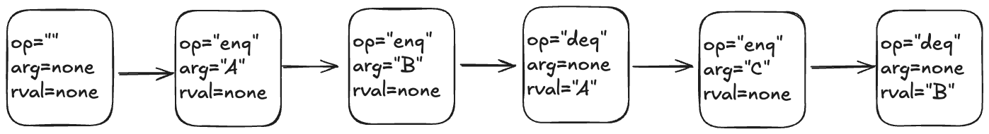
My model uses three state variables:
- op – identifies which operation is being invoked (enq or deq)
- arg – the argument being passed in the case of the enq operation
- rval – the return value in the case of the deq operatoin
TLA+ requires that we specify a value for every variable in every state, which means we need to specify a value for arg even for the deq operation, which doesn’t have an argument, and a value for rval for the enq operation, which doesn’t return a value. I defined a special value called none for this case.
In the first state, when the queue is empty, I chose to set op to the empty string (“”) and arg and rval to none.
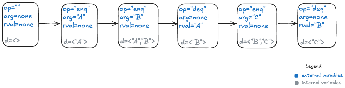
The internal variables
For a queue, we need to keep track all of the values that have previously been enqueued, as well as the order in which they were enqueued.
TLA+ has a type called a sequence which I’ll use to encode this information: a sequence is like a list in Python.
I’ll add a new variable which I’ll unimaginatively call d, for data. Here’s what that behavior looks like with the internal variable.
Modeling dequeues
Recall that our queue supports two operations: enqueue and dequeue. We’ll start with the dequeue operation. I modeled it with an action called Deq.
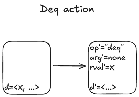
Here are some examples of state transitions that are permitted by the Deq action. We call these Deq steps.

I’m not going to write much TLA+ code in this post, but to give you a feel for it, here is how you would write the Deq action in TLA+ syntax:
Deq == /\ d # <<>>
       /\ op' = "deq"
       /\ arg' = none
       /\ rval' = Head(d)
       /\ d' = Tail(d)
The syntax of the first line might be a bit confusing if you’re not familiar with TLA+:
#is TLA+ for ≠<<>>is TLA+ for the empty sequence.
Modeling dequeues
Here’s what the Enq action looks like:
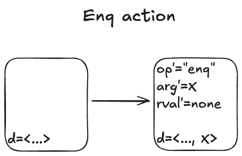
There’s non-determinism in this action: the value of arg’ can be any valid value that we are allowed to put onto the queue.
I’ll spend just a little time in this section to give you a sense of how you would use TLA+ to represent the simple queue model.
To describe the queue in TLA+, we define a set called Values that contains all of the valid values that could be enqueued, as well as a special constant named none that means “not a value”.
CONSTANTS Values, none
ASSUME none \notin Values
Then we would encode the Enq action like this:
Enq == /\ op' = "enq"
       /\ arg' \in Values
       /\ rval' = none
       /\ d' = Append(d, arg')
The complete description of our queue, its specification that describes all permitted behaviors, looks like this:

For completeness, here’s what the TLA+ specification looks like: (source in Queue.tla).
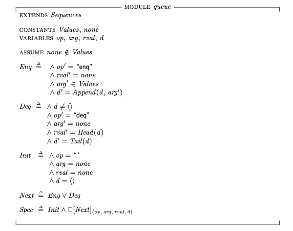
Init corresponds to our set of initial states, and Next corresponds to the next-state action, where the two sub-actions are Enq and Deq.
The last line, Spec, is the full specification. You can read this as: The initial state is chosen from the Init set of states, and every step is a Next step (every allowed state transition is a member of the set of state transitions defined by the Next action).
Modeling concurrency
In our queue model above, an enqueue or dequeue operation happens in one step (state transition). That’s fine for modeling sequential programs, but it’s not sufficient for modeling concurrent programs. In concurrent programs, the operations from two different threads can overlap in time.
To illustrate, imagine a scenario where there are three threads, t1, t2, t3. First, t1 enqueues “A”, and “B”. Then, t2 and t3 both call dequeue, and those queries overlap in time.
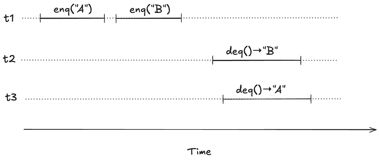
We want to model concurrent executions using a state-machine model. The diagram above, shows the start and end time for each operation. But to model this behavior, we don’t actually care about the exact start and end times: rather, we only care about the relative order of the start and events.
Below shows the threads in different columns.
       t1                t2                t3
---------------   ----------------  ----------------
enq("A") [start]
enq("A") [end]
enq("B") [start]
enq("B") [end]
                  deq() [start]
                                    deq() [start]
                  deq() → "B" [end]
                                    deq() → "A" [end]
Here’s the same execution history, shown in a single column:
t1: enq("A") [start]
t1: enq()    [end]
t1: enq("B") [start]
t1: enq("B") [end]
t2: deq() [start]
t3: deq() [start]
t2: deq() → "B" [end]
t3: deq() → "A" [end]
We can model execution histories like the one above using state machines. We were previously modeling an operation in a single state transition (step). Now we will need to use two steps to model an operation: one to indicate when the operation starts and the other to indicate when the operate ends.
Because each thread acts independently, we need to model variables that are local to threads. And, in fact, all externally visible variables are scoped to threads, because each operation always happens in the context of a particular thread. We do this by changing the variables to be functions where the domain is a thread id. For example, where we previously had op=”enq” where op was always a string, now op is a function that takes a thread id as an argument. Now we would have op[t1]=”enq” where t1 is a thread id. (Functions in TLA+ use square brackets instead of round ones. you can think of these function variables as acting like dictionaries)
Here’s an example of a behavior that models the above execution history, showing only the external variables. Note that this behavior only shows the values that change in a state.
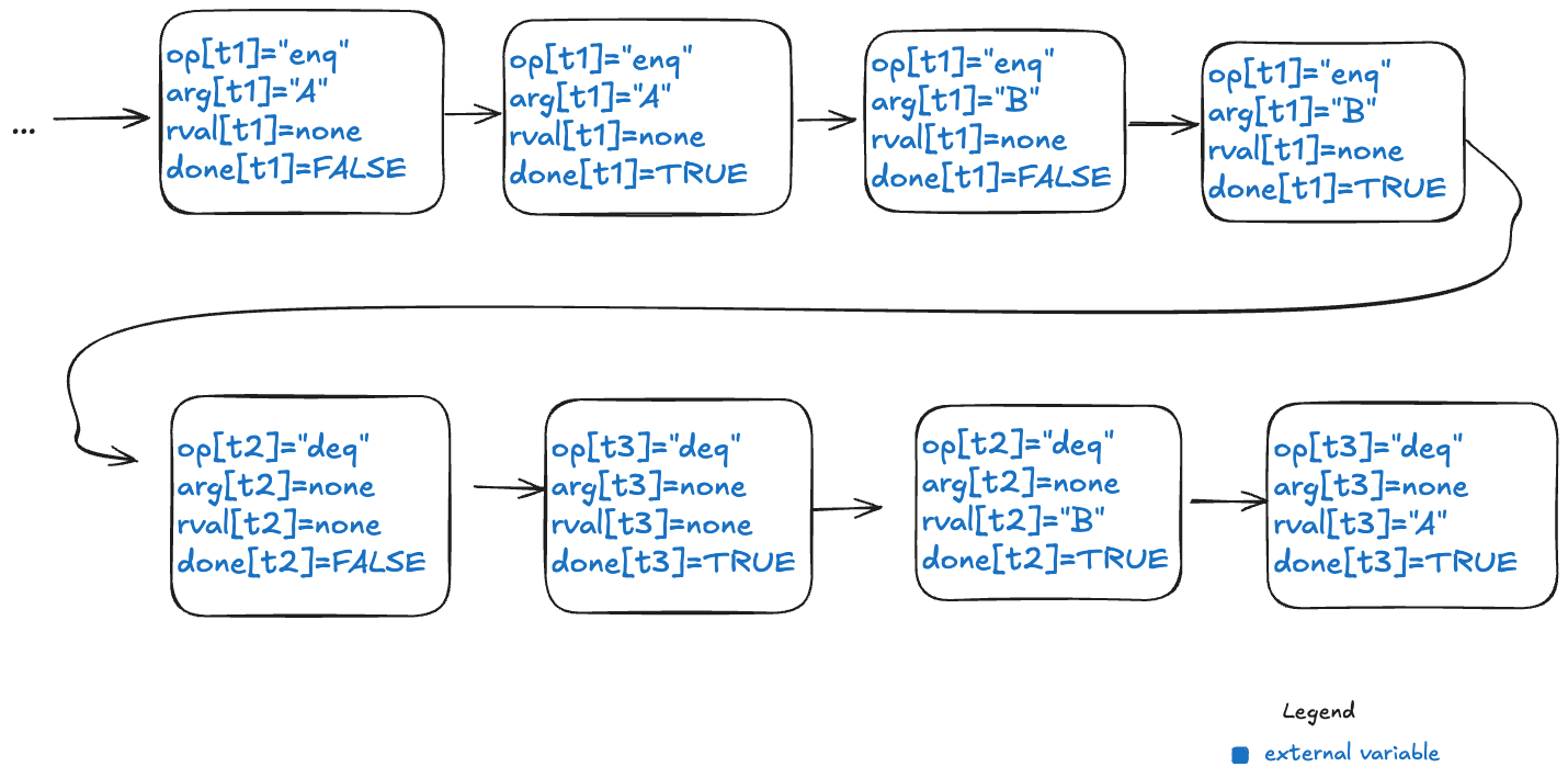
Note the following changes from the previous behaviors.
- There is a boolean flag, done, which indicates when the operation is complete.
- The variables are all scoped to a specific thread.
But what about the internal variable d?
Linearizability as correctness condition for concurrency
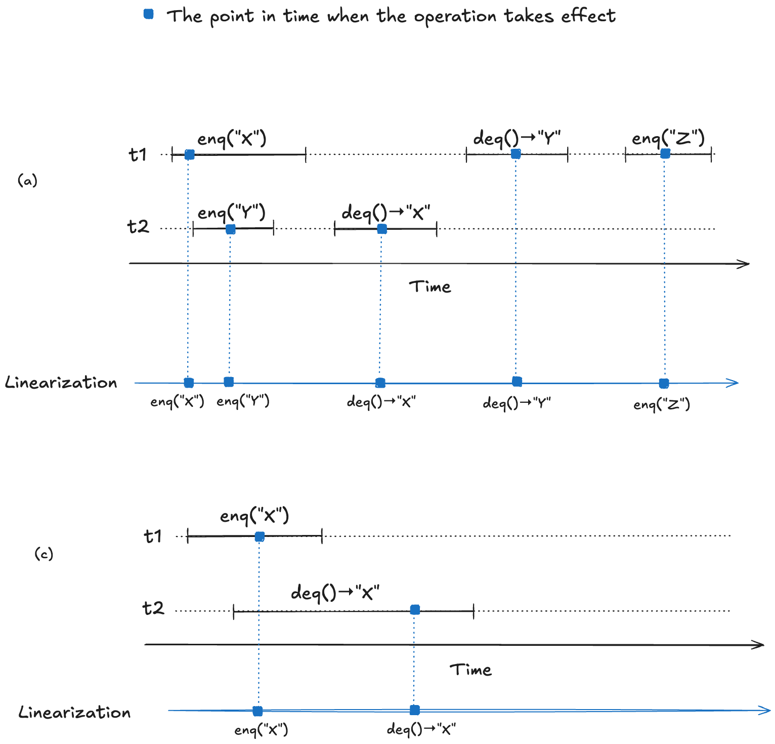
We know what it means for a sequential queue to be correct. But what do we want to consider correct when operations can overlap? We need to decide what it means for an execution history of a queue to be correct in the face of overlapping operations. This is where linearizability comes in. From the abstract of the Herlihy and Wing paper:
Linearizability provides the illusion that each operation applied by concurrent processes takes effect instantaneously at some point between its invocation and its response, implying that the meaning of a concurrent object’s operations can be given by pre- and post-conditions.
For our queue example, we say our queue is linearizable if, for every history where there are overlapping operations, we can identify a point in time between the start and end of the operation where the operation instantaneously “takes effect”, giving us a sequential execution history that is a correct execution history for a serial queue. This is a called a linearization. If every execution history for our queue has a linearization, then we say that our queue is linearizable.
To make this concrete, consider the following four observed execution histories of a queue, labeled (a), (b), (c), (d), adapted from Fig. 1 of the Herlihy and Wing linearizable paper. Two of these histories are linearizable (they are labeled “OK”), and two are not (labeled “NOT OK”).
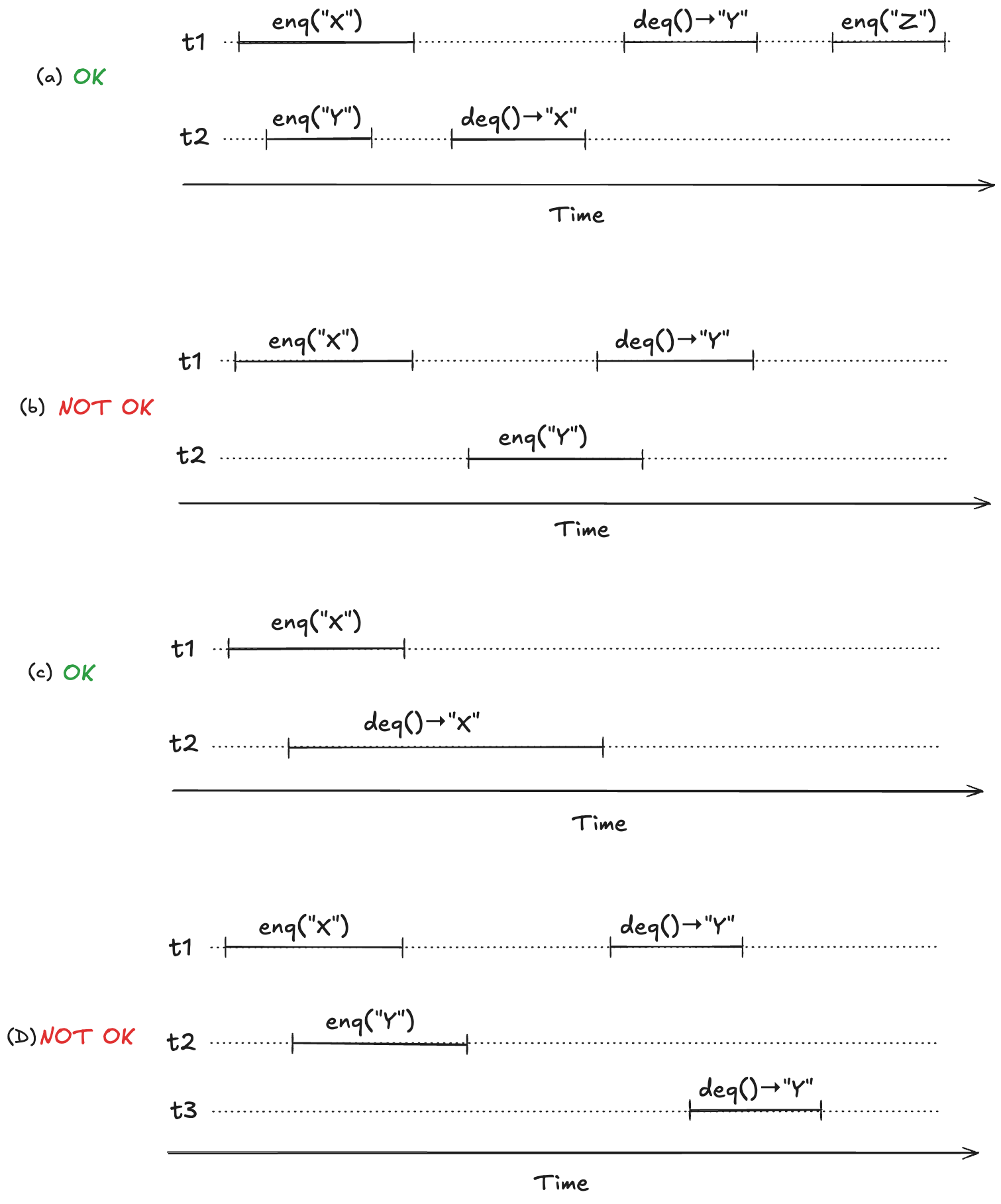
For (a) and (c), we can identify points in time during the operation where it appears as if the operation has instantaneously taken effect.
We now have a strict ordering of operations because there is no overlap, so we can write it as a sequential execution history. When the resulting sequential execution history is valid, it is called a linearization:
(a)
t1: enq("X")
t2: enq("Y")
t2: deq() → "X"
t1: deq() → "Y"
t2: enq("Y")

(b)
t1: enq("X")
t2: deq() → "X"
Modeling a linearizable queue in TLA+
To repeat from the last section, a data structure is linearizable if, for every operation that executes on the data structure, we can identify a point in time between the start and the end of the operation where the operation takes effect.
We can model a linearizable queue by modeling each operation (enqueue/dequeue) as three actions:
- Start (invocation) of operation
- When the operation takes effect
- End (return) of operation
Our model needs to permit all possible linearizations. For example, consider the following two linearizable histories. Note how the start/end timings of the operations are identical in both cases, but the return values are different.
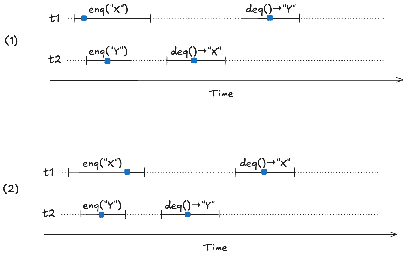
In (1) the first deq operation returns “X”, and in (2) the first deq operation “returns Y”. Yet they are both valid histories. The difference between the two is the order in which the enq operations take effect. In (1), enq(“X”) takes effect before enq(“Y”), and in (2), enq(“Y”) takes effect before enq(“X”). Here are the two linearizations:
(1)
enq("X")
enq("Y")
deq()→"X"
deq()→"Y"

(2)
enq("Y")
enq("X")
deq()→"X"
deq()→"Y"
Our TLA+ model of a linearizable queue will need to be able to model the relative order of when these operations take effect. This is where the internal variables come into play in our model: “taking effect” will mean updating internal variables of our model.
We need an additional variable to indicate whether the internal state has been updated or not for the current operation. I will call this variable up (for “updated”). It starts off as false when the operation starts, and is set to true when the internal state variable (d) has been updated.
Here’s a visual representation of the permitted state transitions (actions). As before, the left bubble shows the values that must be true in the first state for the transition to happen, and the second bubble shows which variables change.
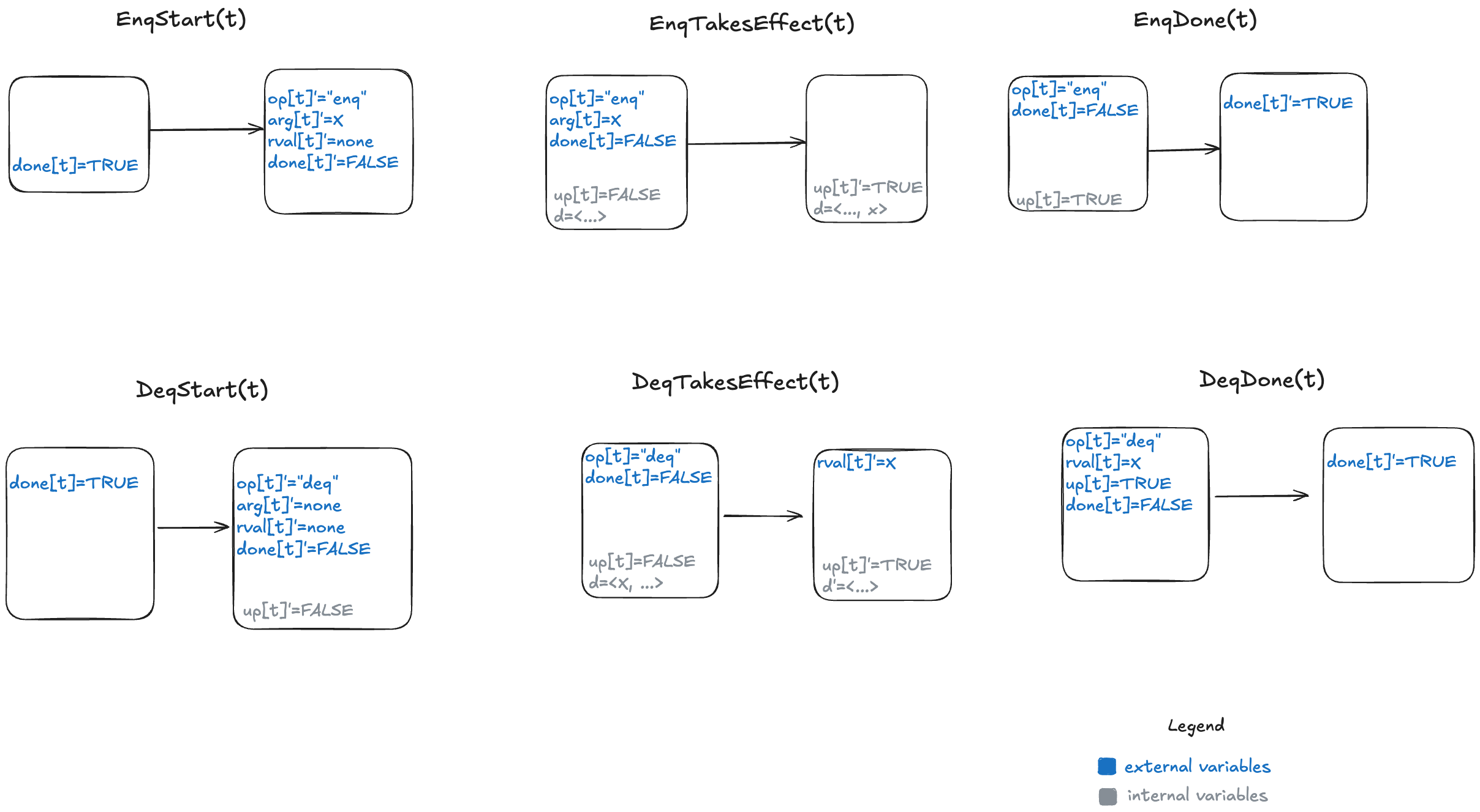
Since we now have to deal with multiple threads, we parameterize our action by thread id (t). You can see the TLA+ model here: LinearizableQueue.tla.
We now have a specification for a linearizable queue, which is a description of all valid behaviors. We can use this to verify that a specific queue implementation is linearizable. To demonstrate, let’s shift gears and talk about an example of an implementation.
An example queue implementation
Let’s consider an implementation of a queue that:
- Stores the data in a doubly-linked list
- Uses a lock to protect the list
A queue with four entries looks like this:
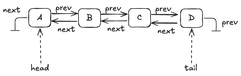
Here’s an implementation of this queue in Python that I whipped up. I call it an “LLLQueue” for “locked-linked-list queue”. I believe that my LLLQueue is linearizable, and I’d like to verify this.
One way is to use TLA+ to build a specification of my LLLQueue, and then prove that every behavior of my LLLQueue is also a behavior of the LinearizableQueue specification. The way we do this is in TLA+ is by a technique called refinement mappings.
But, first, let’s model the LLLQueue in TLA+.
Modeling the LLLQueue in TLA+ (PlusCal)
In a traditional program, a node would be associated with a pointer or reference. I’m going to use numerical IDs for each node, starting with 1. I’ll use the value of 0 as a sentinel value meaning null.
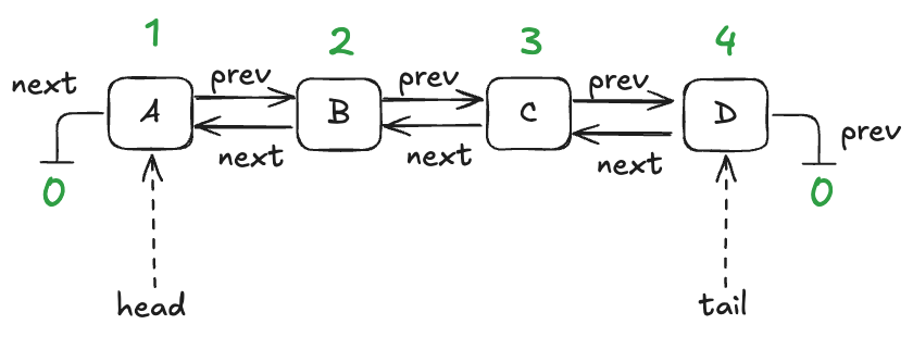
We’ll model this with three functions:
- vals – maps node id to the value stored in the node
- prev – maps node id to the previous node id in the list
- next – maps node id to the next node id in the list
Here are these functions in table form for the queue shown above:
| node id | vals |
|---|---|
| 1 | A |
| 2 | B |
| 3 | C |
| 4 | D |
| node id | prev |
|---|---|
| 1 | 2 |
| 2 | 3 |
| 3 | 4 |
| 4 | 0 (null) |
| node id | next |
|---|---|
| 1 | 0 (null) |
| 2 | 1 |
| 3 | 2 |
| 4 | 3 |
It’s easier for me to use PlusCal to model an LLLQueue than to do it directly in TLA+. PlusCal is a language for specifying algorithms that can be automatically translated to a TLA+ specification.
It would take too much space to describe the full PlusCal model and how it translates, but I’ll try to give a flavor of it. As a reminder, here’s the implementation of the enqueue method in my Python implementation.
    def enqueue(self, val):
        self.lock.acquire()
        new_tail = Node(val=val, next=self.tail)
        if self.is_empty():
            self.head = new_tail
        else:
            self.tail.prev = new_tail
        self.tail = new_tail
        self.lock.release()
Here’s what my PlusCal model looks like for the enqueue operation:
procedure enqueue(val)
variable new_tail;
begin
E1: acquire(lock);
E2: with n \in AllPossibleNodes \ nodes do
        Node(n, val, tail);
        new_tail := n;
    end with;
E3: if IsEmpty then
        head := new_tail;
    else
        prev[tail] := new_tail;
    end if;
    tail := new_tail;
E4: release(lock);
E5: return;
end procedure;
Note the labels (E1, E2, E3, E4, E5) here. The translator turns those labels into TLA+ actions (state transitions permitted by the spec). In my model, an enqueue operation is implemented by five actions.
Refinement mappings
One of the use cases for formal methods is to verify that a (low-level) implementation conforms to a (higher-level) specification. In TLA+, all specs are sets of behaviors, so the way we do this is that we:
- create a high-level specification that models the desired behavior of the system
- create a lower-level specification that captures some implementation details of interest
- show that every behavior of the low-level specification is among the set of behaviors of the higher-level specification, considering only the externally visible variables
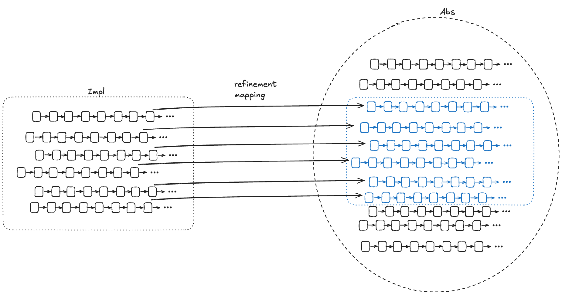
In the diagram below, Abs (for abstract) represents the set of valid (externally visible) behaviors of a high-level specification, and Impl (for implementation) represents the set of valid (externally visible) behaviors for a low-level specification. For Impl to implement Abs, the Impl behaviors must be a subset of the Abs behaviors.
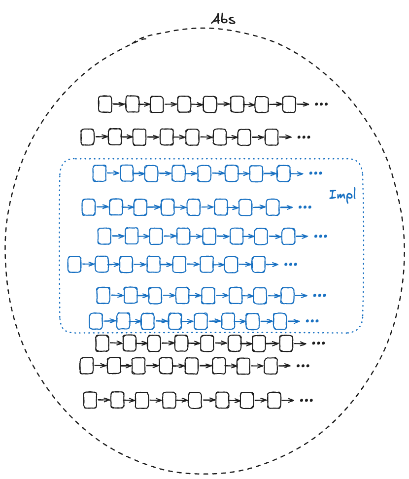
We want to be able to prove that Impl implements Abs. In other words, we want to be able to prove that every externally visible behavior in Impl is also an externally visible behavior in Abs.

One approach is to do this by construction: if we can take any behavior in Impl and construct a behavior in Abs with the same externally visible values, then we have proved that Impl implements Abs.
As Lamport and Abadi put it in their paper The Existence of Refinement Mappings back in 1991:
To prove that S1 implements S2, it suffices to prove that if S1 allows the behavior
<<(e0,z0), (e1, z1), (e2, z2), …>>
where [ei is a state of the externally visible component and] the zi are internal states, then there exists internal states yi such that S2 allows
<<(e0,y0), (e1, y1), (e2, y2), … >>
For each behavior B1 in Impl, if we can find values for internal variables in a behavior of Abs, B2, where the external variables of B2 match the external variables of B1, then that’s sufficient to prove that Impl implements Abs.
To show that Impl implements Abs, we need to find a refinement mapping, which is a function that will map every behavior in Impl to a behavior in Abs.
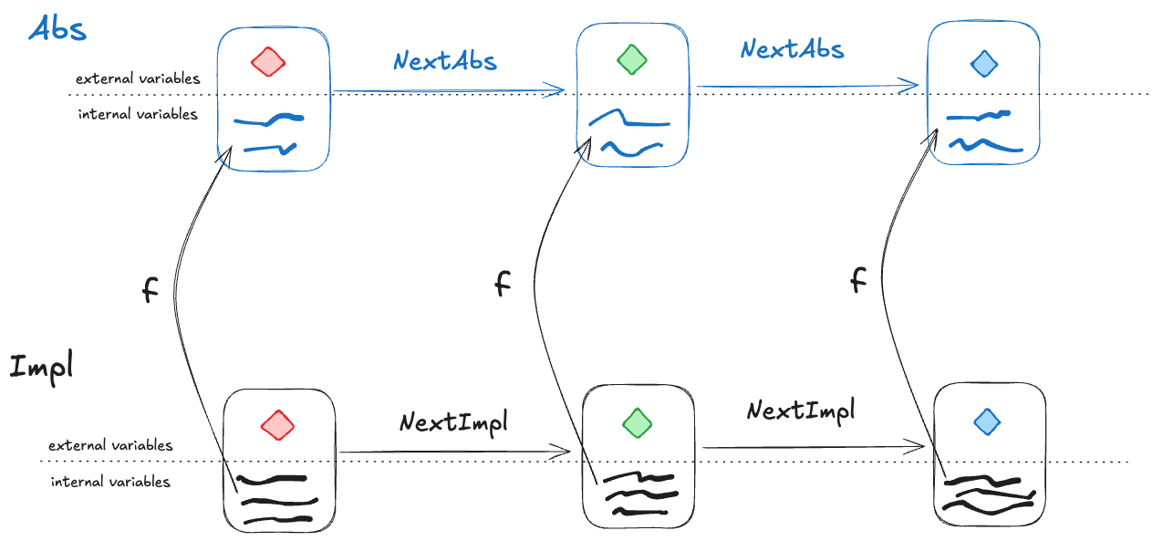
A refinement mapping takes a state in an Impl behavior as input and maps to an Abs state, such that:
- the external variables are the same in both the Impl state and the Abs state
- if a pair of states is a permitted Impl state transition, then the corresponding mapped pair of states must be a permitted Abs state transition
Or, to reword statement 2: if NextImpl is the next-state action for Impl (i.e., the set of allowed state transitions for Impl), and NextAbs is the next-state action for Abs, then under the refinement mapping, every NextImpl-step must map to a NextAbs step.
(Note: this technically isn’t completely correct, we’ll see why in the next section).
Example: our LLLQueue
We want to verify that our Python queue implementation is linearizable. We’ve modeled our Python queue in TLA+ as LLLQueue, and to prove that it’s linearizable, we need to show that a refinement mapping exists between the LLLQueue spec and the LinearizableQueue spec. This means we need to show that there’s a mapping from LLLQueue’s internal variables to LinearizableQueue’s internal variables.

We need to define the internal variables in LinearizableQueue (up, d) in terms of the variables in LLLQueue (nodes, vals, next, prev, head, tail, lock, new_tail, empty, pc, stack) in such a way that all LLLQueue behaviors are also LinearizableQueue behaviors under the mapping.
Internal variable: d
The internal variable d in LinearizableQueue is a sequence which contains the values of the queue, where the first element of the sequence is the head of the queue.
Looking back at our example LLLQueue queue:
We need a mapping that, for this example, results in: d =〈A,B,C,D 〉
I defined a recursive operator that I named Data such that when you call Data(head), it evaluates to a sequence with the values of the queue.
Internal variable: up
The variable up is a boolean flag that flips from false to true after the value has been added to the queue.
In our LLLQueue model, the new node gets added to the tail by the action E3. In PlusCal models, there’s a variable named pc (program counter) that records the current execution state of the program. You can think of pc like a breakpoint that points to the action that will be executed on the next step of the program. We want up to be true after action E3. You can see how the up mapping is defined at the bottom of the LLLQueue.tla file.
Refinement mapping and stuttering
Let’s consider a behavior of the LLLQueue spec that enqueues a single value onto the queue, with a refinement mapping to the LinearizableQueue spec:
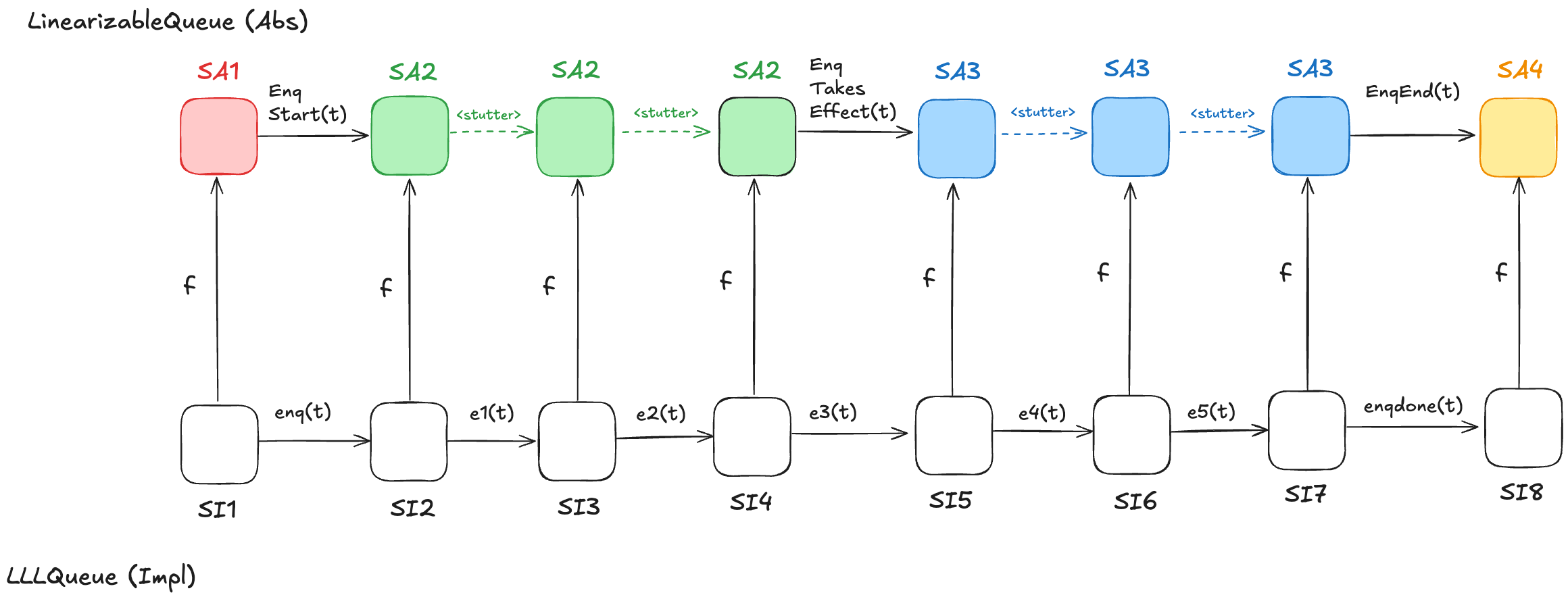
In the LinearizableQueue spec, an enqueue operation is implemented by three actions:
- EnqStart
- EnqTakesEffect
- EnqEnd
In the LLLQueue spec, an enqueue operation is implemented by seven actions: enq, e1, …, e5, enqdone. That means that the LLLQueue enqueue behavior involves eight distinct states, where the corresponding LinearizableQueue behavior involves only four distinct states. Sometimes, different LLLQueue states map to the same LinearizableQueue state. In the figure above, SI2,SI3,SI4 all map to SA2, and SI5,SI6,SI7 all map to SA3. I’ve color-coded the states in the LinearizableQueue behavior such that states that have the same color are identical.
As a result, some state transitions in the refinement mapping are not LinearizableQueue actions, but are instead transitions where none of the variables change at all. These are called stuttering steps. In TLA+, stuttering steps are always permitted in all behaviors.
A problem with refinement mappings: the Herlihy and Wing queue
The last section of the Herlihy and Wing paper describes how to prove that a concurrent data structure’s operations are linearizable. In the process, the authors also point out a problem with refinement mappings. They illustrate the problem using a particular queue implementation, which we’ll call the “Herlihy & Wing queue”, or H&W Queue for short.
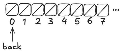
Imagine an array of infinite length, where all of the values are initially null. There’s a variable named back which points to the next available free spot in the queue.
Enqueueing
To enqueue a value onto the Herlihy & Wing queue involves two steps:
- Increment the back variable
- Write the value into the spot where the back variable pointed before being incremented .
Here’s what the queue looks like after three values (A,B,C) have been enqueued:
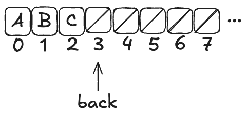
Note how back always points to the next free spot.
Dequeueing
To dequeue, you start at index 0, and then you sweep through the array, looking for the first non-null value. Then you atomically copy that value out of the array and set the array element to null.
Here’s what a dequeue operation on the queue above would look like:
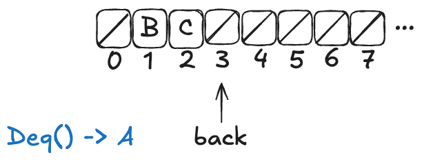
The Deq operation returned A, and the first element in the array has been set to null.
If you were to enqueue another value (say, D), the array would now look like this:

Note: the elements at the beginning of the queue that get set to null after a dequeue don’t get reclaimed. The authors note that this is inefficient, but the purpose of this queue is to illustrate a particular issue with refinement mappings, not to be a practical queue implementation.
H&W Queue pseudocode
Here’s the pseudocode for Herlihy & Wing queue, which I copied directly from the paper. The two operations are Enq (enqueue) and Deq (dequeue).
rep = record {back: int, items: array [item]}

Enq = proc (q: queue, x: item)
  i: int := INC(q.back) % Allocate a new slot
  STORE (q.items[i], x) % Fill it.
  end Enq

Deq = proc (q: queue) returns (item)
  while true do
    range: int := READ(q.back) - 1
    for i: int in 1 .. range do
      x: item := SWAP(q.items[i], null)
      if x ~= null then return(x) end
      end
    end
end Deq
This algorithm relies on the following atomic operations on shared variables:
- INC – atomically increment a variable and return the pre-incremented value
- STORE – atomically write an element into the array
- READ – atomically read an element in the array (copy the value to a local variable)
- SWAP – atomically write an element of an array and return the previous array value
H&W Queue implementation in C++
Here’s my attempt at implementing this queue using C++. I chose C++ because of its support for atomic types. C++’s atomic types support all four of the atomic operations required of the H&W queue.
| Atomic operation | Description | C++ equivalent |
|---|---|---|
| INC | atomically increment a variable and return the pre-incremented value | std::atomic<T>::fetch_add |
| STORE | atomically write an element into the array | std::atomic_store |
| READ | atomically read an element in the array (copy the value to a local variable) | std::atomic_load |
| SWAP | atomically write an element of an array and return the previous array value | std::atomic_exchange |
My queue implementation stores pointers to objects of parameterized type T. Note the atomic types of the member variables. The back variable and elements of the items array need to be atomics because we will be invoking atomic operations on them.
template <typename T>
class Queue {
    atomic<int> back;
    atomic<T *> *items;

public:
    Queue(int sz) : back(0), items(new atomic<T *>[sz]) {}
    ~Queue() { delete[] items; }

    void enq(T *x);
    T *deq();
};

template<typename T>
void Queue<T>::enq(T *x) {
    int i = back.fetch_add(1);
    std::atomic_store(&items[i], x);
}

template<typename T>
T *Queue<T>::deq() {
    while (true) {
        int range = std::atomic_load(&back);
        for (int i = 0; i < range; ++i) {
            T *x = std::atomic_exchange(&items[i], nullptr);
            if (x != nullptr) return x;
        }
    }
}
We can write enq and deq to look more like idiomatic C++ by using the following atomic operators:
- T operator++( int ) instead of fetch_add
- std::atomic::operator= instead of atomic_store
- std::atomic::operator T instead of atomic_load
Using these operators, enq and deq look like this:
template<typename T>
void Queue<T>::enq(T *x) {
    int i = back++;
    items[i] = x;
}

template<typename T>
T *Queue<T>::deq() {
    while (true) {
        int range = back;
        for (int i = 0; i < range; ++i) {
            T *x = std::atomic_exchange(&items[i], nullptr);
            if (x != nullptr) return x;
        }
    }
}
Note that this is, indeed, a linearizable queue, even though it does not use mutual exclusion: tthere are no critical sections in the algorithm.
Modeling the H&W queue in TLA+ with PlusCal
The H&W queue is straightforward to model in PlusCal. If you’re interested in learning PlusCal, it’s actually a great example to use. See HWQueue.tla for my implementation.
Refinement mapping challenge: what’s the state of the queue?
Note how the enq method isn’t an atomic operation. Rather, it’s made up of two atomic operations:
- Increment back
- Store the element in the array
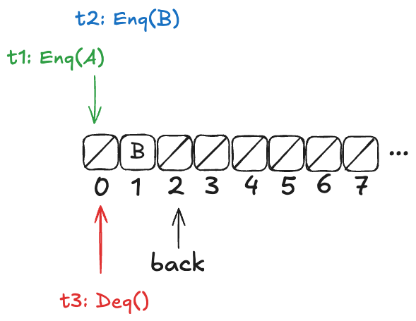
Now, imagine that a thread, t1, comes along, to enqueue a value to the queue. It starts off by incrementing back.
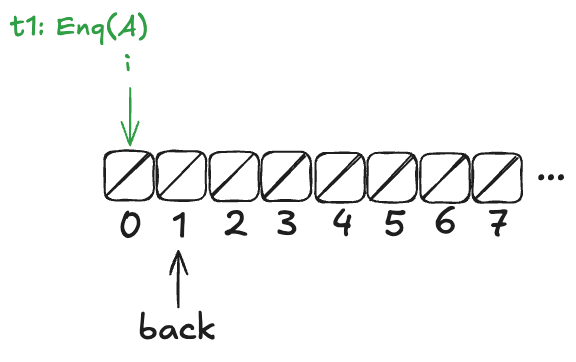
But before it can continue, a new thread, t2, gets scheduled, which also increments back:
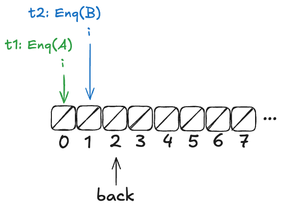
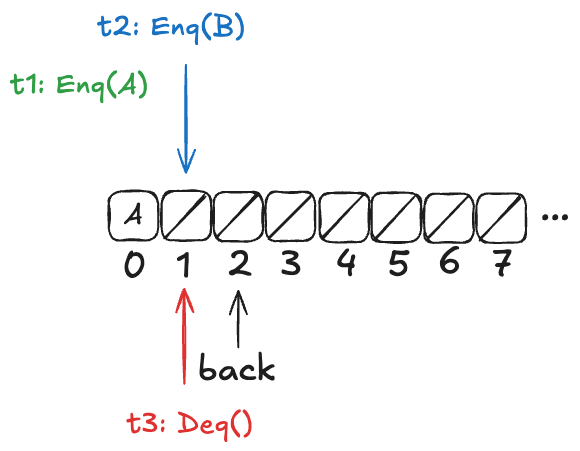
t2 then completes the operation:
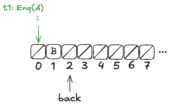
Finally, a new thread, t3, comes along that executes the dequeue operation:
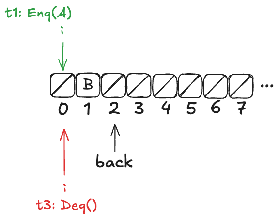
Now, here’s the question: What value will the pending Deq() operation return: A or B?
The answer: it depends on how the threads t1 and t3 will be scheduled. If t1 is scheduled first, it will write A to position 0, and then t3 will read it. On the other hand, if t3 is scheduled first, it will advance its i pointer to the next non-null value, which is position 1, and return B.
Recall back in the section “Modeling a queue with TLA+ > The internal variables” that our model for a linearizable queue had an internal variable, named d, that contained the elements of the queue in the order in which they had been enqueued.
If we were to write a refinement mapping of this implementation to our linearizable specification, for the state above, we’d have to decide whether the mapping for the above state should be. The problem is that no such refinement mapping exists.
Here are the only options that make sense for the example above:
- d =〈B〉
- d =〈A,B〉
- d =〈B,A〉
As a reminder, here are the valid state transitions for the LinearizableQueue spec.

Option 1: d =〈B〉
Let’s say we define our refinement mapping by using the populated elements of the queue. That would result in a mapping of d =〈B〉.
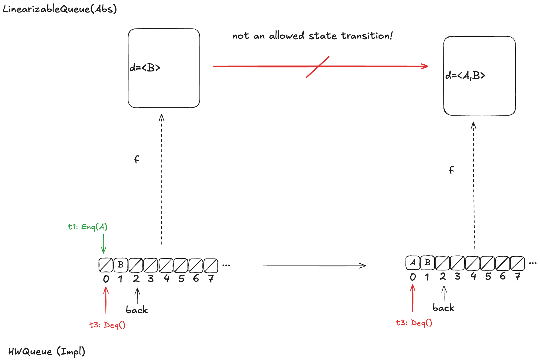
The problem is that if t1 gets scheduled first and adds value A to array position 0, then an element will be added to the head of d. But the only LinearizableQueue action that adds an element to d is EnqTakeEffect, which adds a value to the to the end of d. There is no LinearizableQueue action that allows prepending to d, so this cannot be a valid refinement mapping.
Option 2: d =〈A,B〉
Let’s say we had chosen instead a refinement mapping of d =〈A,B〉for the state above. In that case, if t3 gets scheduled first, then it will result in a value being removed from the end of d, which is not one of the actions of the LinearizableQueueSpec, which means that this can’t be a valid refinement mapping either.

Option 3: d =〈B,A〉
Finally, assume we had chosen d =〈B,A〉as our refinement mapping. Then, if t1 gets scheduled first, and then t3, we will end up with a state transition that removes an element from the end of d, which is not a LinearizableQueue action.
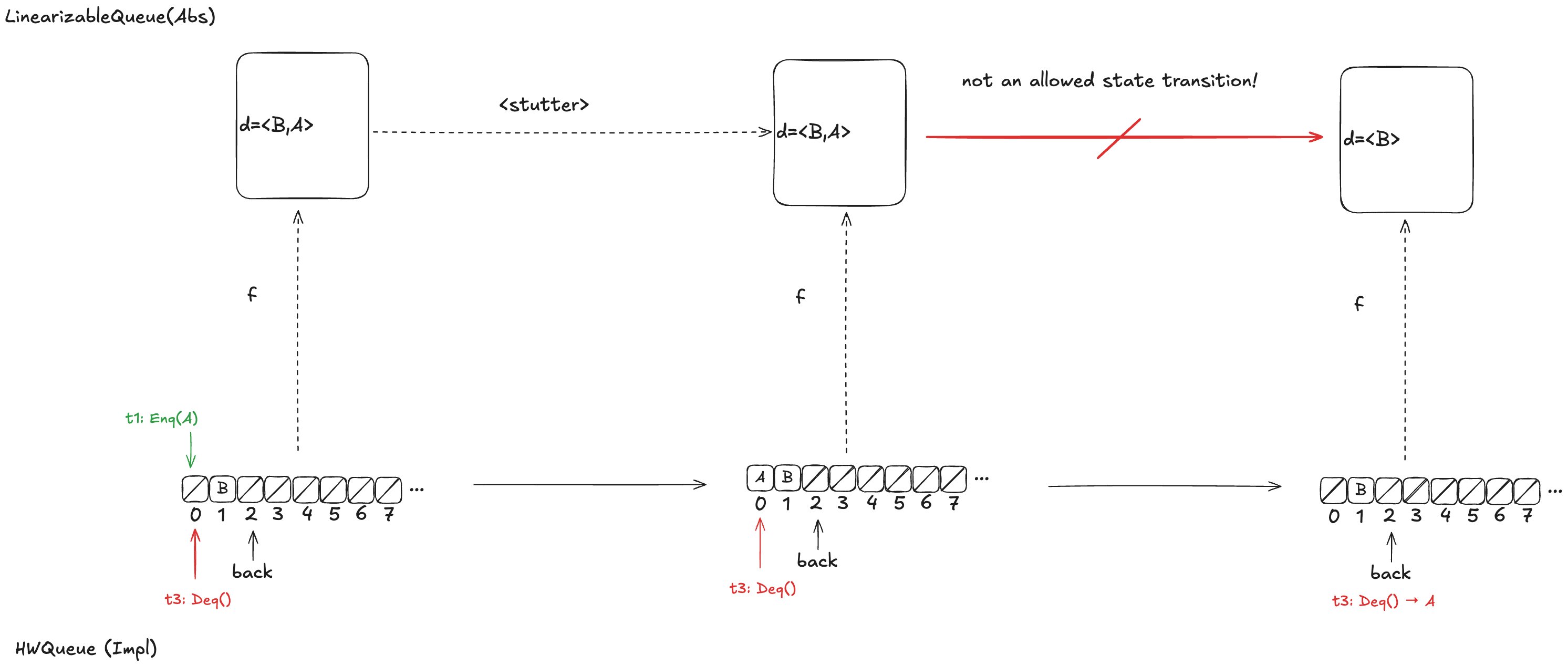
Whichever refinement mapping we choose, it is possible that the resulting behavior will violate the LinearizableQueue spec. This means that we can’t come up with a refinement mapping where every behavior of Impl maps to a valid behavior of Abs, even though Impl implements a linearizable queue!
What Lamport and others believed at the time was that this type of refinement mapping always existed if Impl did indeed implement Abs. With this counterexample, Herlihy & Wing demonstrated that this was not always the case.
Elements in H&W queue aren’t totally ordered
In a typical queue implementation, there is a total ordering of elements that have been enqueued. The odd thing about the Herlihy & Wing queue is that this isn’t the case.
If we look back at our example above:
Either A or B might be dequeued next, depending on the ordering of t1 and t3. Here’s another example where the value dequeued next depends on the ordering of the threads t1 and t3.
However, there are also scenarios where there is a clear ordering among values that have been added to the queue. Consider a case similar to the one above, except that t2 has not yet incremented the back variable:
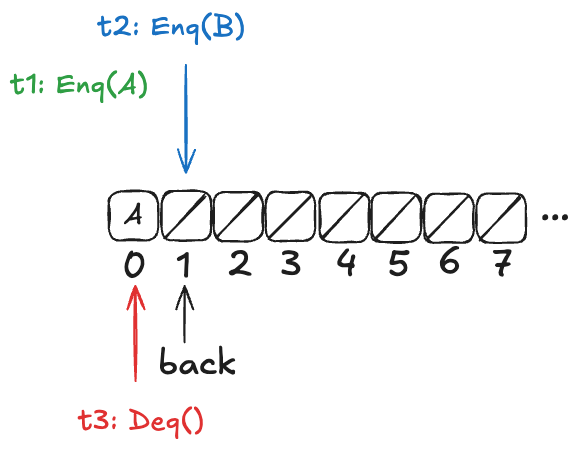
In this configuration, A is guaranteed to be dequeued before B. More generally, if t1 writes A to the array before t2 increments the back variable, then A is guaranteed to be dequeued before B.
In the linearizability paper, Herlihy & Wing use a mapping approach where they identify a set of possible mappings rather than a single mapping.
Let’s think back to this scenario:
In the scenario above, in the Herlihy and Wing approach, the mapping would be to the set of all possible values of queue.
- queue ∈ {〈B〉,〈A,B〉, 〈B,A〉}
Lamport took a different approach to resolving this issue. He rescued the idea of refinement mappings by introducing a concept called prophecy variables
Prophecy
The Herlihy & Wing queue’s behavior is non-deterministic: we don’t know the order in which values will be dequeued, because it depends on the scheduling of the threads. But imagine if we know in advance the order in which the values were dequeued.
It turns out that if we can predict the order in which the values would be dequeued, then we can do a refinement mapping to the our LinearizableQueue model.
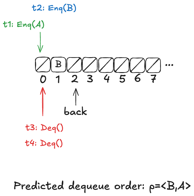
This is the idea behind prophecy variables: we predict certain values that we need for refinement mapping.
Adding a prophecy variable gives us another specification (one which has a new variable), and this is the specification where we can define a refinement mapping. For example, we add a prophecy to our HWQueue model and call the new model HWQueueProphecy.
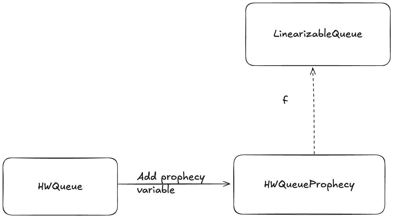
In HWQueueProphecy, we maintain a sequence of the predicted order in which values will be dequeued. Every time a thread invokes the enqueue operation, we add a new value to our sequence of predicted dequeue operations.
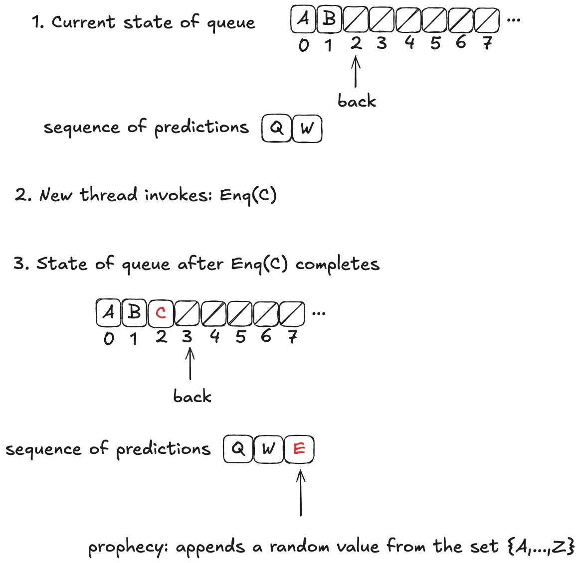
The predicted value is chosen at random from the set of all possible values: it is not necessarily related to either the value currently being enqueued or the current state of the queue.
Now, these predictions might not actually come true. In fact, they almost certainly won’t come true, because we’re much more likely to predict at least one value incorrectly. In the example above, the actual dequeueing order will be〈A,B,C〉, which is different from the predicted dequeueing order of〈Q,W,E〉
However, the refinement mapping will still work, even though the predictions will often be wrong, if we set things up correctly. We’ll tackle that next.
Prophecy requirements
We want to show that HWQueue implements LinearizableQueue. But it’s only HWQueueProphecy that we can show implements LinearizableQueue using a refinement mapping.
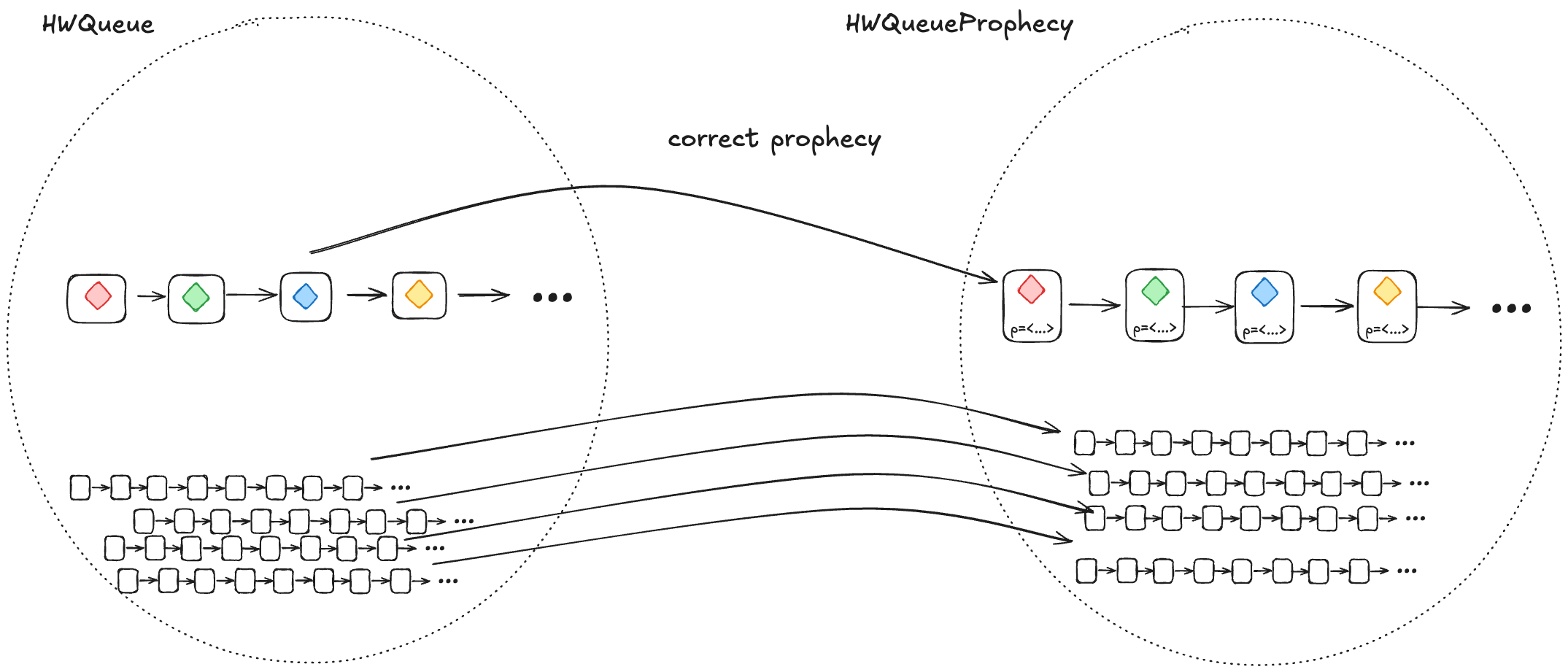
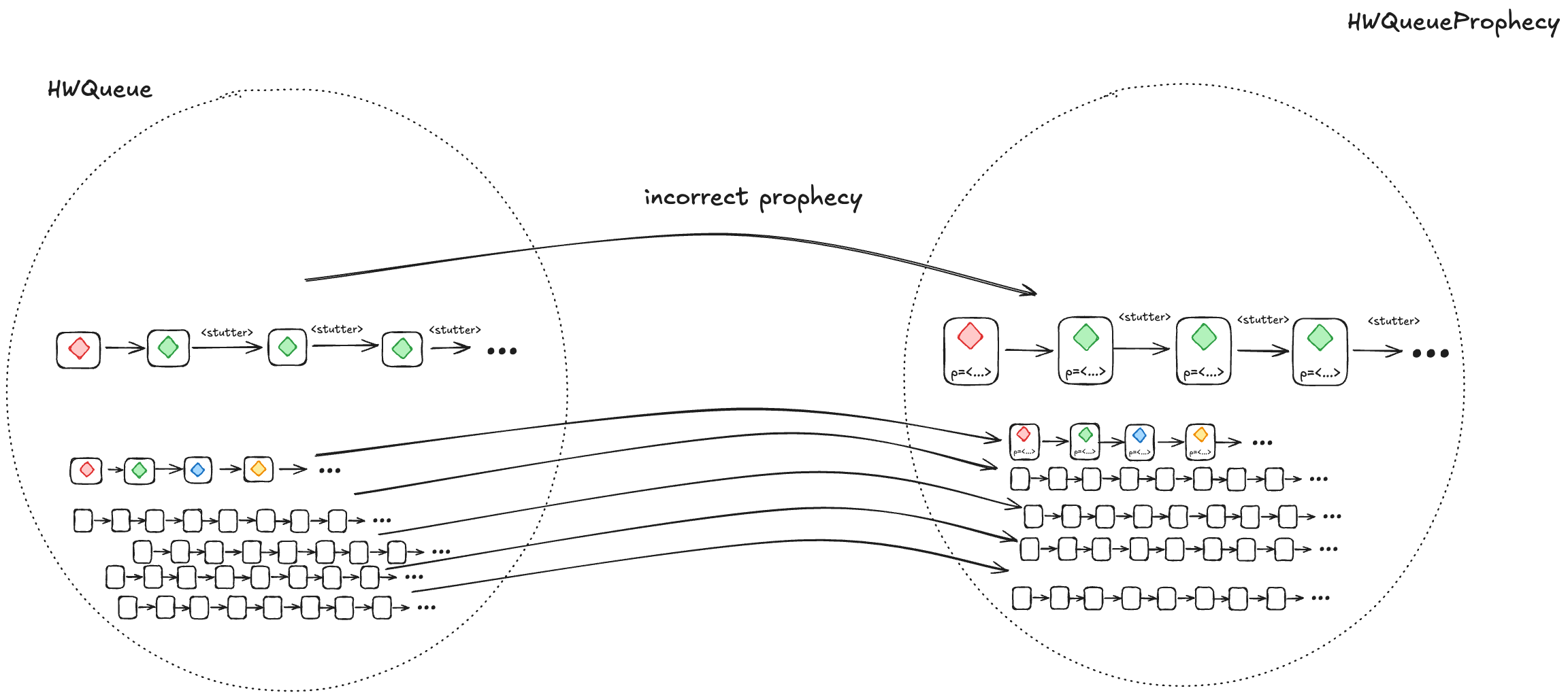
1. A correct prophecy must exist for every HWQueue behavior
Every behavior in HWQueue must have a corresponding behavior in HWQueueProphecy. That correspondence happens when the prophecy accurately predicts the dequeueing order.
This means that, for each behavior in HWQueue, there must be a behavior in HWQueueProphecy which is identical except that the HWQueueProphecy behaviors have an additional p variable with the prophecy.
To ensure that a correct prophecy always exists, we just make sure that we always predict from the set of all possible values.
In the case of HWQueueProphecy, we are always enqueueing values from the set {A,…,Z}, and so as long as we draw predictions from the set {A,…,Z}, we are guaranteed that the correct prediction is among the set we are predicting from.
2. Every HWQueueProphecy behavior with an incorrect prophecy must correspond to at least one HWQueue behavior
Most of the time, our predictions will be incorrect. We need to ensure that, when we prophesize incorrectly, the resulting behavior is still a valid HWQueue behavior, and is also still a valid LinearizableQueue behavior under refinement.
We do this by writing our HWQueueProphecy specification such that, if our prediction turns out to be incorrect (e.g., we predict A as the next value to be dequeued, and the next value that will actually be dequeued is B), we disallow the dequeue from happening.
In other words, we disallow state transitions that would violate our predictions.
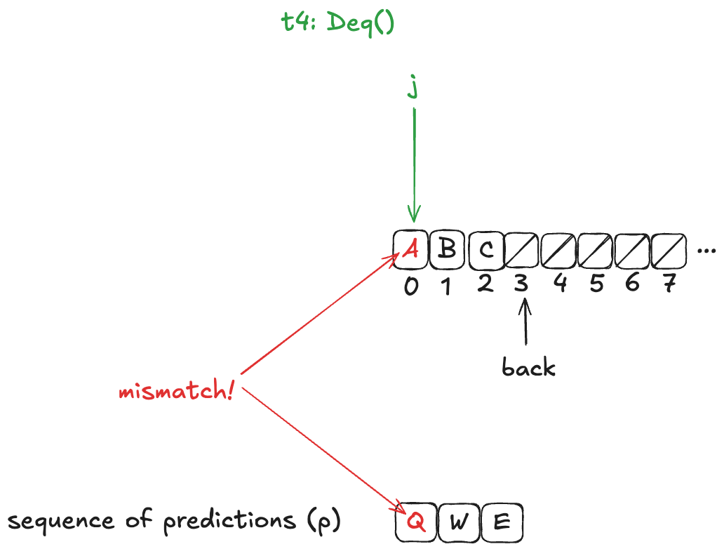
This means we add a new enabling condition to one of the dequeue actions. Now, for the dequeueing thread to remove the value from the array, it has to match the next value in the predicted sequence. In HWQueueProphecy, the name of the action that does this is D5, where t is id of the thread doing the dequeueing.
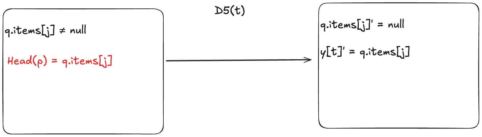
An incorrect prophecy blocks the dequeueing from actually happening. In the case of HWQueueProphecy, we can still enqueue values (since we don’t make any predictions on enqueue order, only dequeue order, so there’s nothing to block).
But let’s consider the more interesting case where an incorrect prophecy results in deadlock, where no actions are enabled anymore. This means that the only possible future steps in the behavior are stuttering steps, where the values never change.
However, if we take a valid behavior of a specification, and we add stuttering steps, the resulting behavior is always also a valid behavior of the specification. So, the resulting behaviors are guaranteed to be in the set of valid HWQueue behaviors.
Using the prophecy to do the refinement mapping
Let’s review what we were trying to accomplish here. We want to figure out a refinement mapping from HWQueueProphecy to LinearizableQueue such that every state transition satisfies the LinearizableQueue specification.
Here’s an example, where the value B has been enqueued, the value A is in the process of being enqueued, and no values have been dequeued yet.
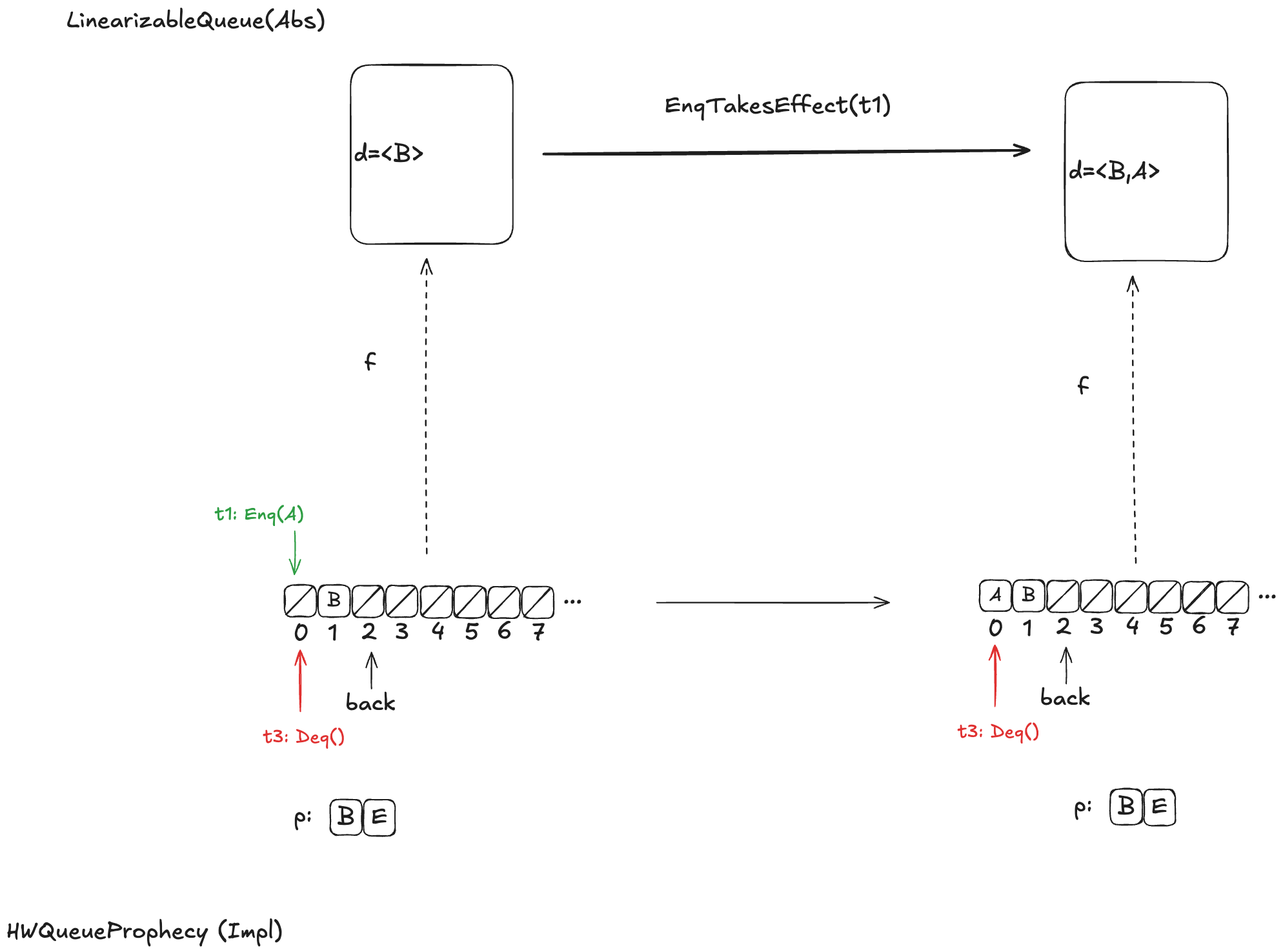
Defining how to do this mapping is not obvious, and I’m not going to explain it here, as it would take up way too much space, and this post is already much too long. Instead, I will defer interested readers to section 6.5 of Lamport’s book A Science of Concurrent Programs, which describes how to do the mapping. See also my POFifopq.tla spec, which is my complete implementation of his description.
But I do want to show you something about it.
Enqueue example
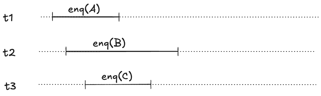
Let’s consider this HWQueue behavior, where we are concurrently enqueueing three values (A,B,C):
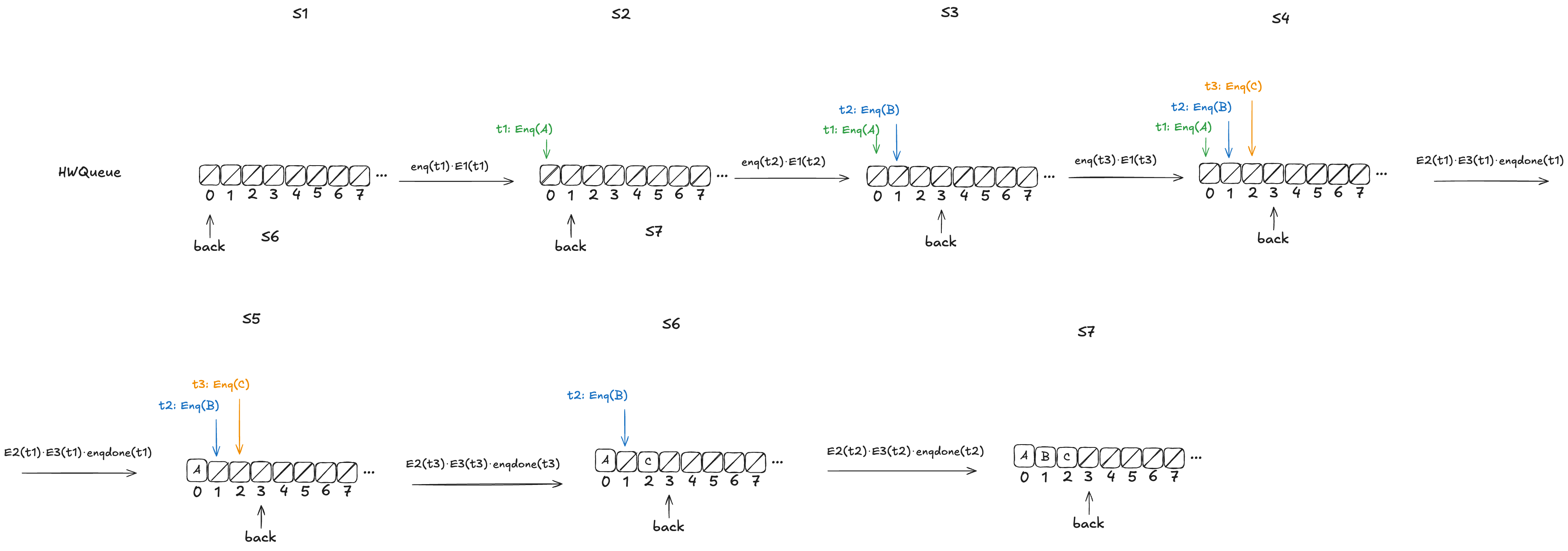
These enqueue operations all overlap each other, like this:
The refinement mapping will depend on the predictions.
Here’s an example where the predictions are consistent with the values being enqueued. Note how the state of the mapping ends up matching the predicted values.
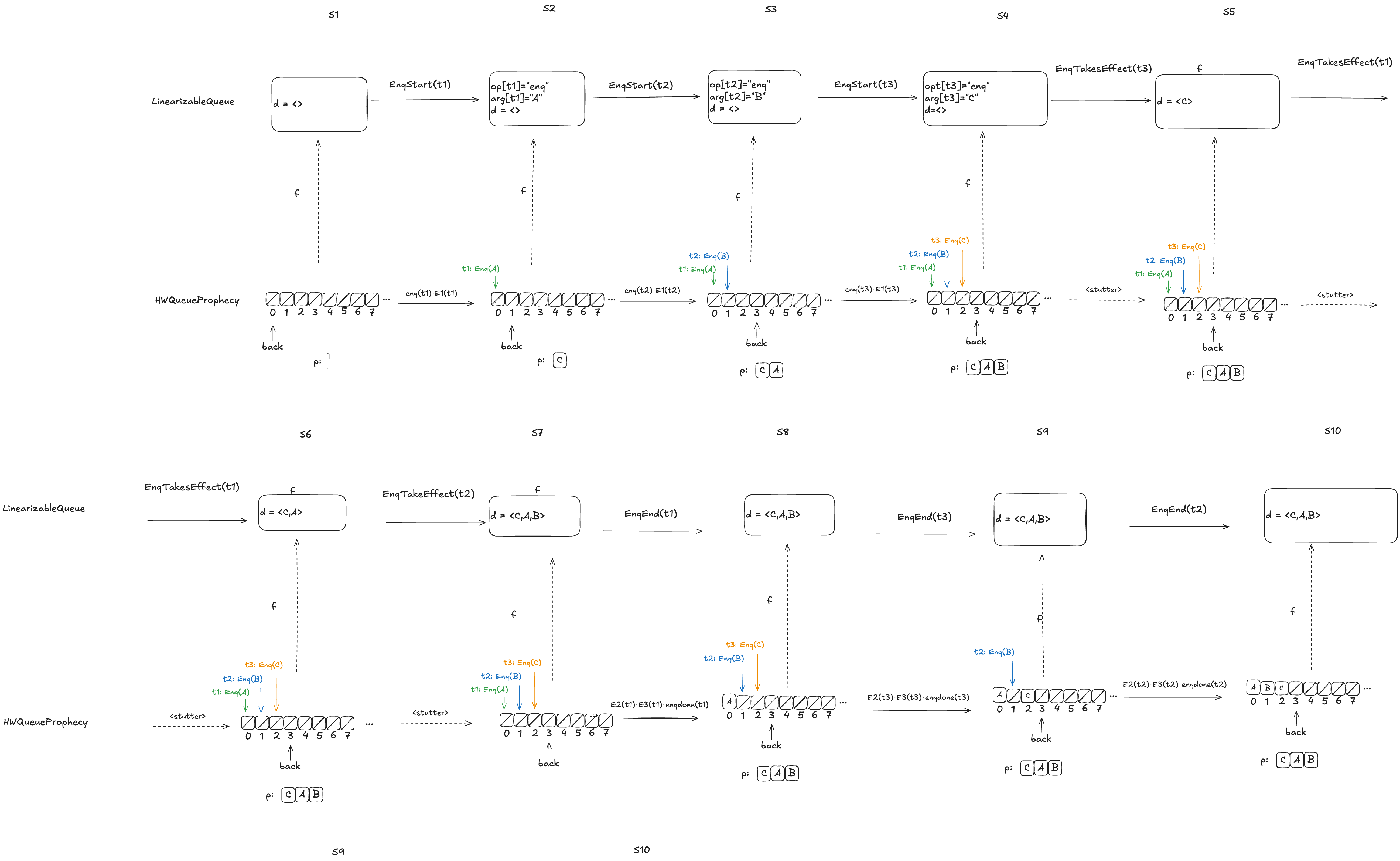
Notice how in the final state (S10), the refinement mapping d=〈C,A,B〉is identical to the predicted dequeue ordering: p=〈C,A,B〉.
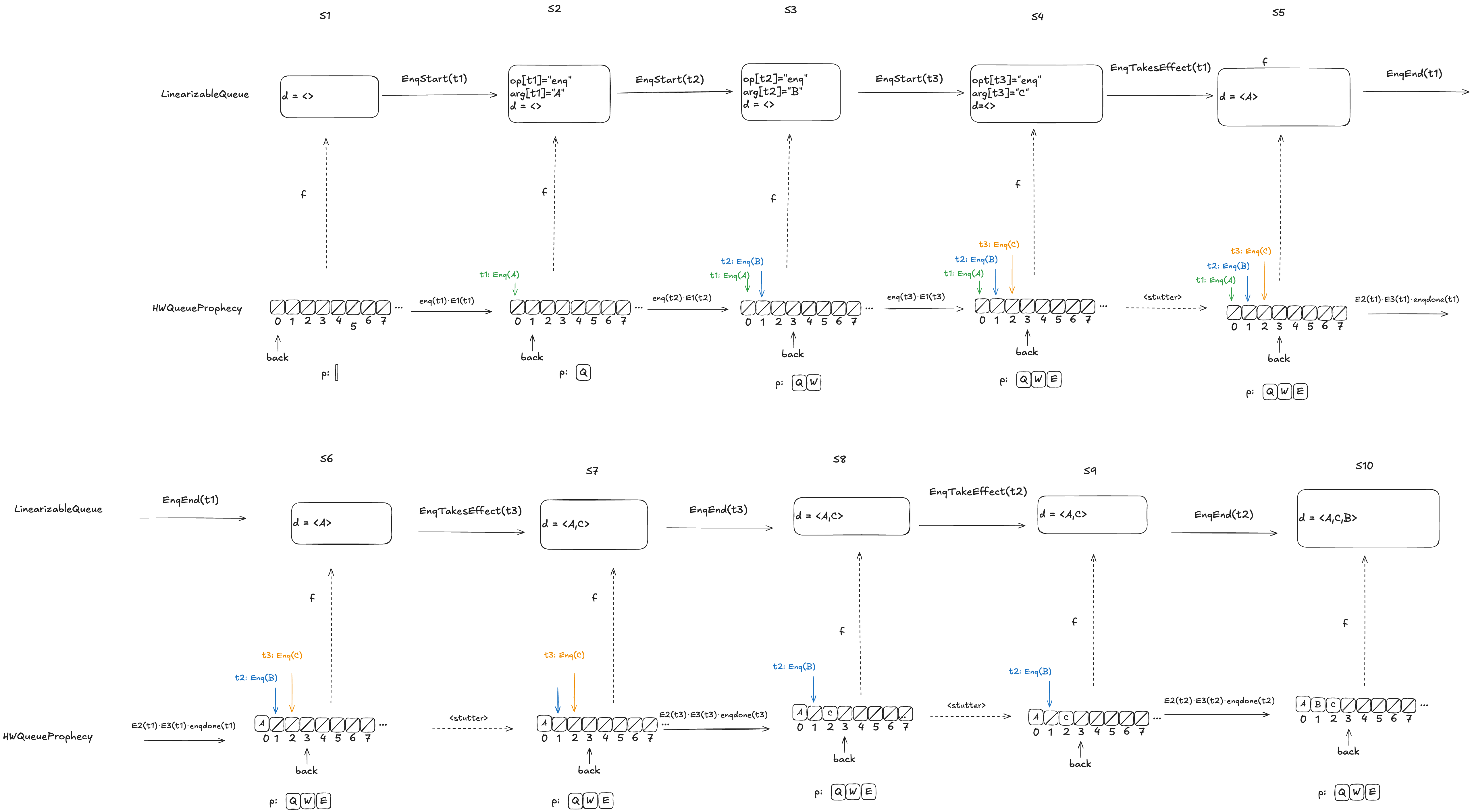
Here the predicted dequeue values p=〈Q,W,E〉can never be fulfilled, and the refinement mapping in this case, d=〈A,C,B〉matches the order in which overlapping enqueue operations complete.
The logic for determining the mapping varies depending on whether it is possible for the predictions to be fulfilled. For more details on this, see A Science of Concurrent Programs.
For the dequeueing case, if the value to be dequeued matches the first prediction in p, then we execute the dequeue and we remove the prediction from p. (We’ve already discussed the behavior if the value to be dequeued doesn’t match the prediction).
Coda
Phew! There was a lot of content in this post, including definitions and worked out examples. It took me a long time to grok a lot of this material, so I suspect that even an interested reader won’t fully absorb it on the first read. But if you got all of the way here, you’re probably interested enough in TLA+ that you’ll continue to read further on it. I personally find that it helps to have multiple explanations and examples, and I’ve tried to make an effort to present these concepts a little differently than other sources, so hopefully you’ll find it useful to come back here after reading elsewhere.
The TLA+ models and Python and C++ code are all available in my GitHub tla-prophecy repo.
References
There’s a ton of material out there, much of it papers.
Blog posts
Linearizability: A Correctness Condition for Concurrent Objects, Murat Demirbas, August 9, 2024. This was the post that originally inspired this blog post.
Specification Refinement, Hillel Wayne, July 13, 2021. An explanation of refinement mapping.
Papers
Linearizability: a correctness condition for concurrent objects. Maurice P. Herlihy, Jeannette M. Wing. ACM Transactions on Programming Languages and Systems (TOPLAS), Volume 12, Issue 3, July 1990. This is the paper that introduced linearizability.
Leslie Lamport has a complete list of his papers on his website. But here are a few that are most directly relevant to this post.
A Simple Approach to Specifying Concurrent Systems. Leslie Lamport. Communications of the ACM, Volume 32, Issue 1, January 1989. This paper is a gentle introduction to the transition-axiom method: Lamport’s state-machine method of specifications.
Existence of refinement mappings. Martin Abadi, Leslie Lamport. Proceedings of the 3rd Annual Symposium on Logic in Computer Science. July 1988. This is the paper that introduced the idea of of refinement mapping.
Prophecy Made Simple. Leslie Lamport, Stephan Merz. ACM Transactions on Programming Languages and Systems (TOPLAS), Volume 44, Issue 2, April 2022. This paper is an introduction to the idea of prophecy variables.
Books (PDFs)
A Science of Concurrent Programs. Leslie Lamport. This is a self-published book on how to use TLA to model concurrent algorithms. This book documents how to use prophecy variables to implement the refinement mapping for the linearizable queue in the Herlihy and Wing paper.
A PlusCal User’s Manual. P-Syntax. Version 1.8. Leslie Lamport. 11 March 2024. This is a good general reference for the PlusCal language.
Websites
Learn TLA+. Hillel Wayne. Website with TLA+ learning materials. A good place to start learning TLA+.
The TLA+ Home Page. The official TLA+ website
Consistency Models. Linearizability is a consistency models, but there are multiple other ones. Kyle Kingsbury provides a good overview of the different models on his Jepsen site.
GitHub repositories
https://github.com/lorin/tla-prophecy – This repo contains the actual refinement mappings for the Herlihy & Wing queue. Much of it is transcribed from A Science of Concurrent Programs.
https://github.com/lorin/tla-linearizability – This repo contains my TLA+ models the formal definition of linearizability from the Herlihy & Wing paper.
Edits:
- fixed errors in counter execution history and “Example of Deq steps” diagram
- Fixed typo: transition-axiom not transition-axion

One thought on “Linearizability! Refinement! Prophecy!”