Formal specs as sets of behaviors

Amazon’s recent announcement of their spec-driven AI tool, Kiro, inspired me to write a blog post on a completely unrelated topic: formal specifications. In particular, I wanted to write about how a formal specification is different from a traditional program. It took a while for this idea to really click in my own head, and I wanted to motivate some intuition here.

In particular, there have been a number of formal specification tools that have been developed in recent years which use programming-language-like notation, such as FizzBee, P, PlusCal, and Quint. I think these notations are more approachable for programmers than the more set-theoretic notation of TLA+. But I think the existence of programming-language-like formal specification languages makes it even more important to drive home the difference between a program and a formal spec.

The summary of this post is: a program is a list of instructions, a formal specification is a set of behaviors. But that’s not very informative on its own. Let’s get into it.

What kind of software do we want to specify

Generally speaking, we can divide the world of software into two types of programs. There is one type where you give the program a single input, and it produces a single output, and then it stops. The other type is one that runs for an extended period of time and interacts with the world by receiving inputs over time, and generating outputs over time. In a paper published in the mid 1980s, the computer scientists David Harel (developer of statecharts) and Amir Pneuli (the first person to apply temporal logic to software specifications) made a distinction between programs they called transformational (which is like the first kind) and the another which they called reactive.

Source: On the Development of Reactive Systems by Harel and Pnueli

A compiler is an example of a transformational tool, but you can think of many command-line tools as falling into this category. An example of the second type is the flight control software in an airplane, which runs continuously, taking in inputs and generating outputs over time. In my world, we call services are a great example of reactive systems. They’re long-running programs that receive requests as inputs and generate responses as outputs. The specifications that I’m talking about here apply to the more general reactive case.

A motivating example: a counter

Let’s consider the humble counter as an example of a system whose behavior we want to specify. I’ll describe what operations I want my counter to support using Python syntax:

class Counter:
  def inc() -> None:
    ...
  def get() -> int:
    ...
  def reset() -> None:
    ...

My example will be sequential to keep things simple, but all of the concepts apply to specifying concurrent and distributed systems as well. Note that implementing a distributed counter is a common system design interview problem.

Behaviors

Above I just showed the method signatures, but I implemented this counter and interacted with it in the Python REPL, here’s what that looked like:

>>> c = Counter()
>>> c.inc()
>>> c.inc()
>>> c.inc()
>>> c.get()
3
>>> c.reset()
>>> c.inc()
>>> c.get()
1

People sometimes refer to the sort of thing above by various names: a session, an execution, an execution history, an execution trace. The formal methods people refer to this sort of thing as a behavior, and that’s the term that we’ll use in the rest of this post. Specifications are all about behaviors.

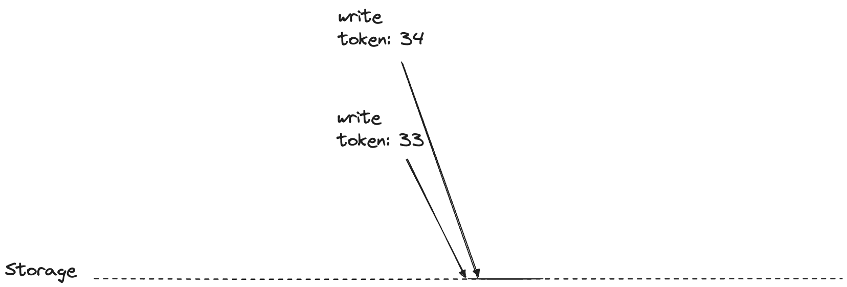
Sometimes I’m going to draw behaviors in this post. I’m going to denote a behavior as a squiggle.

To tie this back to the discussion about reactive systems, you can think of method invocation as inputs, and return values as outputs. The above example is a correct behavior for our counter. But a behavior doesn’t have to be correct: a behavior is just an arbitrary sequence of inputs and outputs. Here’s an example of an incorrect behavior for our counter.

>>> c = Counter()
>>> c.inc()
>>> c.get()
4

We expected the get method to return 1, but instead it returned 4. If we saw that behavior, we’d say “there’s a bug somewhere!”

Specifications and behaviors

What we want out of a formal specification is a device that can answer the question: “here’s a behavior: is it correct or not?”. That’s what a formal spec is for a reactive system. A formal specification is an entity such that, given a behavior, we can determine whether the behavior satisfies the spec. Correct = satisfies the specification.

Once again, a spec is a thing that will tell us whether or not a given behavior is correct.

A spec as a set of behaviors

I depicted a spec in the diagram above as, literally, a black box. Let’s open that box. We can think of a specification simply as a set that contains all of the correct behaviors. Now, the “correct?” processor above is just a set membership check: all it does it check if behavior is an element of the set spec.

What could be simpler?

Note that this isn’t a simplification: this is what a formal specification is in a system like TLA+. It’s just a set of behaviors: nothing more, nothing less.

Describing a set of behaviors

You’re undoubtedly familiar with sets. For example, here’s a set of the first three positive natural numbers: \{1,2,3\}. Here, we described the set by explicitly enumerating each of the elements.

While the idea of a spec being a set of behaviors is simple, actually describing that set is trickier. That’s because we can’t explicitly enumerate the elements of the set like we did above. For one thing, each behavior is, in general, of infinite length. Taking the example of our counter, one valid behavior is to just keep calling any operation over and over again, ad infinitum.

>>> c = Counter()
>>> c.get()
0
>>> c.get()
0
>>> c.get()
0
... (forever)

A behavior of infinite length

This is a correct behavior for our counter, but we can’t write it out explicitly, because it goes on forever.

The other problem is that the specs that we care about typically contain an infinite number of behaviors. If we take the case of a counter, for any finite correct behavior, we can always generate a new correct behavior by adding another inc, get, or reset call.

So, even if we restricted ourselves to behaviors of finite length, if we don’t restrict the total length of a behavior (i.e., if our behaviors are finite but unbounded, like natural numbers), then we cannot define a spec by explicitly enumerating all of the behaviors in the specification.

And this is where formal specification languages come in: they allow us to define infinite sets of behaviors without having to explicitly enumerate every correct behavior.

Describing infinite sets by generating them

Mathematicians deal with infinite sets all of the time. For example, we can use set-builder notation to describe the infinitely large set of all even natural numbers without explicitly enumerating each one:

\{2k \mid k \in \mathbb{N}\}

The example above references another infinite set, the set of natural numbers (ℕ). How do we generate that infinite set without reference to another one?

One way is to define the set by describing how to generate the set of natural numbers. To do this, we specify:

  1. an initial natural number (either 0 or 1, depending on who you ask)
  2. a successor function for how to generate a new natural number from an existing one

This allows us to describe the set of natural numbers without having to enumerate each one explicitly. Instead, we describe how to generate them. If you remember your proofs by induction from back in math class, this is like defining a set by induction.

Specifications as generating a set of behaviors

A formal specification language is just a notation for describing a set of behaviors by generating them. In TLA+, this is extremely explicit. All TLA+ have two parts:

  • Init – which describes all valid initial states
  • Next – which describes how to extend an existing valid behavior to one or more new valid behavior(s)

Here’s a visual representation of generating correct behaviors for the counter.

Generating all correct behaviors for our counter

Note how in the case of the counter, there’s only one valid initial state in a behavior: all of the correct behaviors start the same way. After that, when generating a new behavior based on a previous one, whether one behavior or multiple behaviors can be generated depends on the history. If the last event was a method invocation, then there’s only one valid way to extend that behavior, which is the expected response of the request. If the last event was a return of a method, then you can extend the behavior in three different ways, based on the three different methods you can call on the counter.

The (Init, Next) pair describe all of the possible correct behaviors of the counters by generating them.

Nondeterminism

One area where formal methods can get confusing for newcomers is that the notation for writing the behavior generator can look like a programming language, particularly when it comes to nondeterminism.

When you’re writing a formal specification, you want to express “here are all of the different ways that you can validly extend this behavior”, hence you get that branching behavior in the diagram in the previous section: you’re generating all of the possible correct behaviors. In a formal specification, when we talk about “nondeterminism”, we mean “there are multiple ways a correct behavior can be extended”, and that includes all of the different potential inputs that we might receive from outside. In formal specifications, nondeterminism is about extending a correct behavior along multiple paths.

On the other hand, in a computer program, when we talk about code being nondeterministic, we mean “we don’t know which path the code is going to take”. In the programming world, we typically use nondeterminism to refer to things like random number generation or race conditions. One notable area where they’re different is that formal specifications treat inputs as a source of nondeterminism, whereas programmers don’t include inputs when they talk about nondeterminism. If you said “user input is one of the sources of nondeterminism”, a formal modeler would nod their head, and a programmer would look at you strangely.

Properties of a spec: sets of behaviors

I’ve been using the expressions correct behavior and behavior satisfies the specification interchangeably. However, in practice, we build formal specifications to help us reason about the correctness of the system we’re trying to build. Just because we’ve written a formal specification doesn’t mean that the specification is actually correct! That means that we can’t treat the formal specification that we build as the correct description of the system in general.

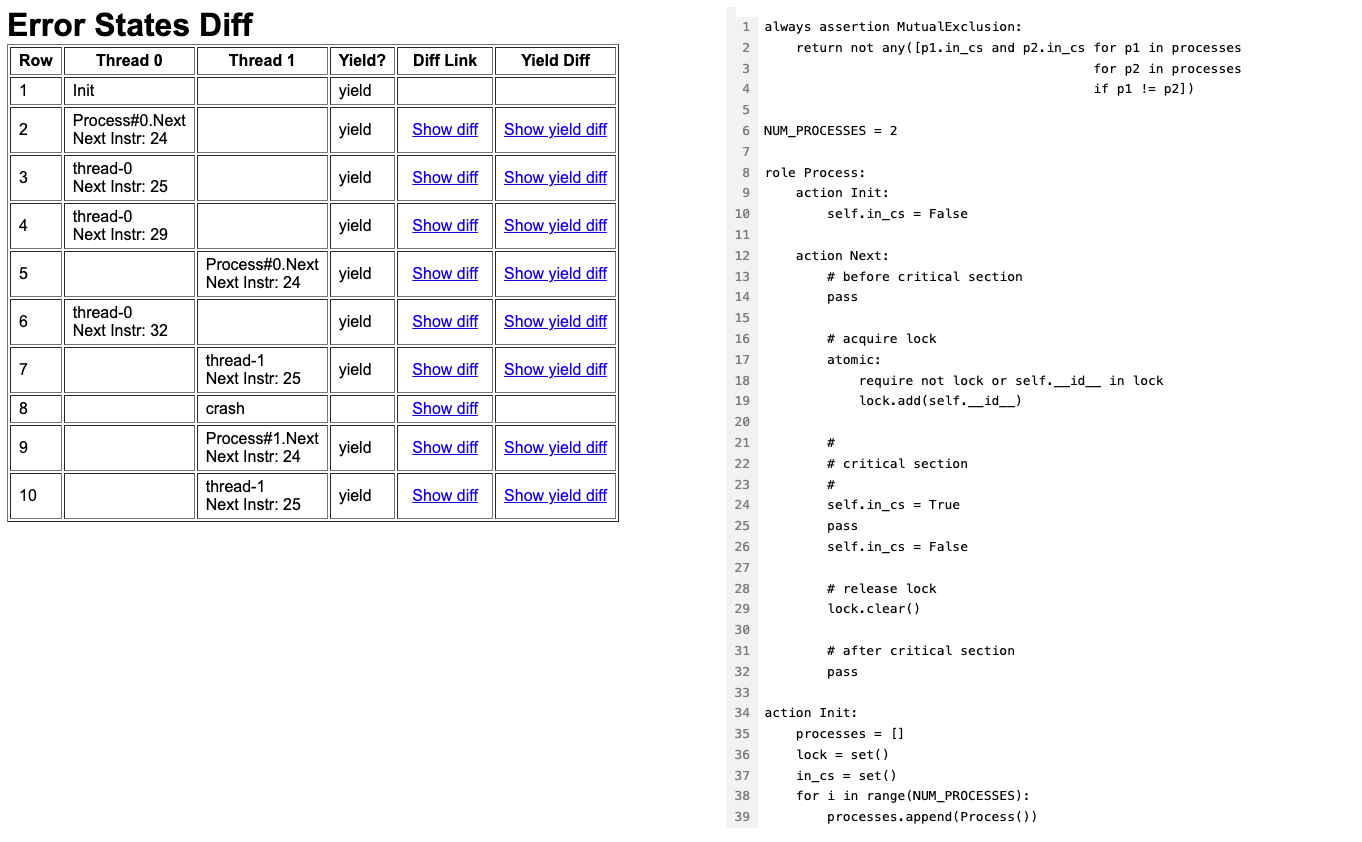
The most frequent tactic people use to reason about their formal specifications is to define correctness properties and use a model-checking tool to check whether their specification conforms to the property or not.

Here’s an example of a property for our counter: the get operation always returns a non-negative value. Let’s give it a name: the no-negative-gets property. If our specification has this property, we don’t know for certain it’s correct. But if it doesn’t have this property, we know for sure something is wrong!

Like a formal specification, a property is nothing more than a set of behaviors! Here’s an example of a behavior that satisfies the no-negative-gets property:

>>> c = Counter()
>>> c.get()
0
>>> c.inc()
>>> c.get()
1

And here’s another one:

>>> c = Counter()
>>> c.get()
5
>>> c.inc()
>>> c.get()
3

Note that the second wrong probably looks wrong to you. We haven’t actually written out a specification for our counter in this post, but if we did, the behavior above would certainly violate it: that’s not how counters work. On the other hand, it still satisfies the no-negative-gets property. In practice, the set of behaviors defined by a property will include behaviors that aren’t in the specification, as depicted below.

A spec that satisfies a property.

When we check that that a spec satisfies a property, we’re checking that Spec is a subset of Property. We just don’t care about the behaviors that are in the Property set but not in the Spec set. What we care about are behaviors that are in Spec that are not in Property. That tells us that our specification can generate behaviors that do not possess the property that we care about.

A spec that does not satisfy a property

Consider the property: get always return a positive number. We can call it all-positive-gets. Note that zero is not considered a positive number. Assuming our counter specification starts at zero, here’s a behavior that violates the all-positive-gets property:

>>> c = Counter()
>>> c.get()
0

Thinking in sets

When writing formal specifications, I found that thinking in terms of sets of behaviors was a subtle but significant mind-shift from thinking in terms of writing traditional programs. Where it helped me most is in making sense of the errors I get when debugging my TLA+ specifications using the TLC model checker. After all, it’s when things break is when you really need to understand whats’s going on under the hood. And I promise you, when you write formal specs, things are going to break. That’s why we write them, to find where the breaks are.

Models, models every where, so let’s have a think

If you’re a regular reader of this blog, you’ll have noticed that I tend to write about two topics in particular:

  1. Resilience engineering
  2. Formal methods

I haven’t found many people who share both of these interests.

At one level, this isn’t surprising. Formal methods people tend to have an analytic outlook, and resilience engineering people tend to have a synthetic outlook. You can see the clear distinction between these two perspectives in the transcript of Leslie Lamport’s talk entitled The Future of Computing: Logic or Biology. Lamport is clearly on the side of the logic, so much so that he ridicules the very idea of taking a biological perspective on software systems. By contrast, resilience engineering types actively look to biology for inspiration on understanding resilience in complex adaptive systems. A great example of this is the late Richard Cook’s talk on The Resilience of Bone.

And yet, the two fields both have something in common: they both recognize the value of creating explicit models of aspects of systems that are not typically modeled.

You use formal methods to build a model of some aspect of your software system, in order to help you reason about its behavior. A formal model of a software system is a partial one, typically only a very small part of the system. That’s because it takes effort to build and validate these models: the larger the model, the more effort it takes. We typically focus our models on a part of the system that humans aren’t particularly good at reasoning about unaided, such as concurrent or distributed algorithms.

The act of creating and explicit model and observing its behavior with a model checker gives you a new perspective on the system being modeled, because the explicit modeling forces you to think about aspects that you likely wouldn’t have considered. You won’t say “I never imagined X could happen” when building this type of formal model, because it forces you to explicitly think about what would happen in situations that you can gloss over when writing a program in a traditional programming language. While the scope of a formal model is small, you have to exhaustively specify the thing within the scope you’ve defined: there’s no place to hide.

Resilience engineering is also concerned with explicit models, in two different ways. In one way, resilience engineering stresses the inherent limits of models for reasoning about complex systems (c.f., itsonlyamodel.com). Every model is incomplete in potentially dangerous ways, and every incident can be seen through the lens of model error: some model that we had about the behavior of the system turned out to be incorrect in a dangerous way.

But beyond the limits of models, what I find fascinating about resilience engineering is the emphasis on explicitly modeling aspects of the system that are frequently ignored by traditional analytic perspectives. Two kinds of models that come up frequently in resilience engineering are mental models and models of work.

A resilience engineering perspective on an incident will look to make explicit aspects of the practitioners’ mental models, both in the events that led up to that incident, and in the response to the incident. When we ask “How did the decision make sense at the time?“, we’re trying to build a deeper understanding of someone else’s state of mind. We’re explicitly trying to build a descriptive model of how people made decisions, based on what information they had access to, their beliefs about the world, and the constraints that they were under. This is a meta sort of model, a model of a mental model, because we’re trying to reason about how somebody else reasoned about events that occurred in the past.

A resilience engineering perspective on incidents will also try to build an explicit model of how work happens in an organization. You’ll often heard the short-hand phrase work-as-imagined vs work-as-done to get at this modeling, where it’s the work-as-done that is the model that we’re after. The resilience engineering perspective asserts that the documented processes of how work is supposed to happen is not an accurate model of how work actually happens, and that the deviation between the two is generally successful, which is why it persists. From resilience engineering types, you’ll hear questions in incident reviews that try to elicit some more details about how the work really happens.

Like in formal methods, resilience engineering models only get at a small part of the overall system. There’s no way we can build complete models of people’s mental models, or generate complete descriptions of how they do their work. But that’s ok. Because, like the models in formal methods, the goal is not completeness, but insight. Whether we’re building a formal model of a software system, or participating in a post-incident review meeting, we’re trying to get the maximum amount of insight for the modeling effort that we put in.

Paxos made visual in FizzBee

Unfortunately, Paxos is quite difficult to understand, in spite of numerous attempts to make it more approachable. — Diego Ongaro and John Ousterhout, In Search of an Understandable Consensus Algorithm.

In fact, [Paxos] is among the simplest and most obvious of distributed algorithms. — Leslie Lamport, Paxos Made Simple.

I was interested in exploring FizzBee more, specifically to play around with its functionality for modeling distributed systems. In my previous post about FizzBee, I modeled a multithreaded system where coordination happened via shared variables. But FizzBee has explicit support for modeling message-passing in distributed systems, and I wanted to give that a go.

I also wanted to use this as an opportunity to learn more about a distributed algorithm that I had never modeled before, so I decided to use it to model Leslie Lamport’s Paxos algorithm for solving the distributed consensus problem. Examples of Paxos implementations in the wild include Amazon’s DynamoDB, Google’s Spanner, Microsoft Azure’s Cosmos DB, and Cassandra. But it has a reputation of being difficult to understand.

You can see my FizzBee model of Paxos at https://github.com/lorin/paxos-fizzbee/blob/main/paxos-register.fizz.

What problem does Paxos solve?

Paxos solves what is known as the consensus problem. Here’s how Lamport describes the requirements for conensus.

Assume a collection of processes that can propose values. A consensus algorithm ensures that a single one among the proposed values is chosen. If no value is proposed, then no value should be chosen. If a value has been chosen, then processes should be able to learn the chosen value.

I’ve always found the term chosen here to be confusing. In my mind, it invokes some agent in the system doing the choosing, which implies that there must be a process that is aware of which value is the chosen consensus value once it the choice has been made. But that isn’t actually the case. In fact, it’s possible that a value has been chosen without any one process in the system knowing what the consensus value is.

One way to verify that you really understand a concept is to try to explain it in different words. So I’m going to recast the problem to implementing a particular abstract data type: a single-assignment register.

Single assignment register

A register is an abstract data type that can hold a single value. It supports two operations: read and write. You can think of a register like a variable in a programming language.

A single assignment register that can only be written to once. Once a client writes to the register, all future writes will fail: only reads will succeed. The register starts out with a special uninitialized value, the sort of thing we’d represent as NULL in C or None in Python.

If the register has been written to, then a read will return the written value.

Only one write can succeed against a single assignment register. In this example, it is the “B” write that succeeds.

Some things to note about the specification for our single assignment register:

  • We doesn’t say anything about which write should succeed, we only care that at most one write succeeds.
  • The write operations don’t return a value, so the writers don’t receive information about whether the write succeeded. The only way to know if a write succeeded is to perform a read.

Instead of thinking of Paxos as a consensus algorithm, you can think of it as implementing a single assignment register. The chosen value is the value where the write succeeds.

I used Lamport’s Paxos Made Simple paper as my guide for modeling the Paxos algorithm. Here’s the mapping between terminology used in that paper and the alternate terminology that I’m using here.

Paxos Made Simple paperSingle assignment register (this blog post)
choosing a valuequorum write
proposerswriters
acceptorsstorage nodes
learnersreaders
accepted proposallocal write
proposal numberlogical clock

As a side note: if you ever wanted to practice doing a refinement mapping with TLA+, you could take one of the existing TLA+ Paxos models and see if you can define a refinement mapping to a single assignment register.

Making our register fault-tolerant with quorum write

One of Paxos’s requirements is that it is fault tolerant. That means a solution that implements a single assignment register using a single node isn’t good enough, because that node might fail. We need multiple nodes to implement our register:

Our single assignment register must be implemented using multiple nodes. The red square depicts a failed node.

If you’ve ever used a distributed database like DynamoDB or Cassandra, then you’re likely familiar with how they use a quorum strategy, where a single write or read may resulting in queries against multiple database nodes.

You can think of Paxos as implementing a distributed database that consists of one single assignment register, where it implements quorum writes.

The way these writes work are:

  1. The writer selects a quorum of nodes to attempt to write to: this is a set of nodes that must contain at least a majority. For example, if the entire cluster contains five nodes, then a quorum must contain at least three.
  2. If the writer attempts to write to every node in the quorum it has selected.

In Lamport’s original paper that introduced Paxos, The Part-Time Parliament, he showed a worked out example of a Paxos execution. Here’s that figure, with some annotations that I’ve added to describe it in terms of a single assignment quorum write register.

In this example, there are five nodes in the cluster, designated by Greek letters {Α,Β,Γ,Δ,Ε}.

The number (#) column acts as a logical clock, we’ll get to that later.

The decree column shows the value that a client attempts to write. In this example, there are two different values that clients attempt to write: {α,β}.

The quorum and voters columns indicate which nodes are in the quorum that the writer selected. A square around a node indicates that the write succeeded against that node. In this example, a quorum must contain at least three nodes, though it can have more than three: the quorum in row 5 contains four nodes.

Under this interpretation, in the first row, the write operation with the argument α succeeded on node Δ: there was a local write to node Δ, but there was not yet a quorum write, as it only succeeded on one node.

While the overall algorithm implements a single assignment register, the individual nodes themselves do not behave as single assignment registers: the value written to a node in can potentially change during the execution of the Paxos algorithm. In the example above, in row 27, the value β is successfully written to node Δ, which is different from the value α written to that node in row 2.

Safety condition: can’t change a majority

The write to our single assignment register occurs when there’s a quorum write: when a majority of the nodes have the same value written to them. To enforce single assignment, we cannot allow a majority of nodes to see a different written value over time.

Here’s how I expressed that safety condition in FizzBee, where written_values is a history variable that keeps track of which values were successfully written to a majority of nodes.

# Only a single value is written
always assertion SingleValueWritten:
    return len(written_values)<=1

Here’s an example scenario that would violate that invariant:

In this scenario, there are three nodes {a,b,c} and two writers. The first writer writes the value x to nodes a and b. As a consequence, x is the value written to the majority of nodes. The second writer writes the value y to nodes b and c, and so y becomes the value written to the majority of nodes. This means that the set of values written is: {x, y}. Because our single assignment register only permits one value to be registered, the algorithm must ensure that a scenario like this does not occur.

Paxos uses two strategies to prevent writes that could change the majority:

  1. Read-before-write to prevent clobbering a known write
  2. Unique, logical timestamps to prevent concurrent writes

Read before write

In Paxos, a writer will first do a read against all of the nodes in its quorum. If any node already contains a write, the writer will use the existing written value.

In the first phase, writer 2 reads a value x from node b. In phase 2, it writes x instead of y to avoid changing the majority.

Preventing concurrent writes

The read-before-write approach works if writer 2 tries to do a write after writer 1 has completed its write. But if the writes overlap, then this will not prevent one writer from clobbering the other writer’s quorum write:

Writer 2 clobbers writer 1’s write on node b because the writer 2’s write had not happened yet when writer 1 did its read.

Paxos solves this by using a logical clock scheme to ensure that only one concurrent writer can succeed. Note that Lamport doesn’t refer to it as a logical clock, but I found it useful to think of it this way.

Each writer has a local clock which is set to a different value. When the writer makes read or write calls, It passes the time of the clock as an additional argument.

Each storage node keeps a logical clock. This storage node’s clock is updated by a read call: if the timestamp of the read call is later than the storage node’s local clock, then the node will advance its clock to match the read timestamp. The node will reject writes with timestamps that are dated before its clock.

Node b reject writer 2’s write

In the example above, node b rejects writer 1’s write because the write has a timestamp of 1, and node b has a logical clock value of 2. As a consequence, a quorum write only occurs when writer 2 completes its write.

Readers

The writes are the interesting part of Paxos, which is where I focused. In my FizzBee model, I chose the simplest way to implement readers: a pub-sub approach where each node publishes out each successful write to all of the readers.

A simple reader implementation is to broadcast each local write to all of the readers.

The readers then keep a tally of the writes that have occurred on each node, and when they identify a majority, they record it.

Modeling with FizzBee

For my FizzBee model, I defined three roles:

  1. Writer
  2. StorageNode
  3. Reader

Writer

There are two phases to the writes. I modeled each phase as an action. Each writer uses its own identifier, __id__, as the value to be written. This is the sort of thing you’d do when using Paxos to do leader election.

role Writer:
    action Init:
        self.v = self.__id__
        self.latest_write_seen = -1
        self.quorum = genericset()

    action Phase1:
        unsent = genericset(storage_nodes)
        while is_majority(len(unsent)):
            node = any unsent
            response = node.read_and_advance_clock(self.clock)
            (clock_advanced, previous_write) = response
            unsent.discard(node)

            require clock_advanced
            atomic:
                self.quorum.add(node)
                if previous_write and previous_write.ts > self.latest_write_seen:
                    self.latest_write_seen = previous_write.ts
                    self.v = previous_write.v

    action Phase2:
        require is_majority(len(self.quorum))
        for node in self.quorum:
            node.write(self.clock, self.v)

One thing that isn’t obvious is that there’s a variable named clock that gets automatically injected into the role when the instance is created in the top-level Init action:

action Init:
    writers = []
    ...
    for i in range(NUM_WRITERS):
        writers.append(Writer(clock=i))

This is how I ensured that each writer had a unique timestamp associated with it.

StorageNode

The storage node needs to support two RPC calls, one for each of the write phases:

  1. read_and_advance_clock
  2. write

It also has a helper function named notify_readers, which does the reader broadcast.

role StorageNode:
    action Init:
        self.local_writes = genericset()
        self.clock = -1

    func read_and_advance_clock(clock):
        if clock > self.clock:
            self.clock = clock

        latest_write = None

        if self.local_writes:
            latest_write = max(self.local_writes, key=lambda w: w.ts)
        return (self.clock == clock, latest_write)


    atomic func write(ts, v):
        # request's timestamp must be later than our clock
        require ts >= self.clock

        w = record(ts=ts, v=v)
        self.local_writes.add(w)
        self.record_history_variables(w)

        self.notify_readers(w)

    func notify_readers(write):
        for r in readers:
            r.publish(self.__id__, write)

There’s a helper function I didn’t show here called record_history_variables, which I defined to record some data I needed for checking invariants, but isn’t important for the algorithm itself.

Reader

Here’s my FizzBee model for a reader. Note how it supports one RPC call, named publish.

role Reader:
    action Init:
        self.value = None
        self.tallies = genericmap()
        self.seen = genericset()

    # receive a publish event from a storage node
    atomic func publish(node_id, write):
        # Process a publish event only once per (node_id, write) tuple
        require (node_id, write) not in self.seen
        self.seen.add((node_id, write))

        self.tallies.setdefault(write, 0)
        self.tallies[write] += 1
        if is_majority(self.tallies[write]):
            self.value = write.v

Generating interesting visualizations

I wanted to generate a trace where there a quorum write succeeded but not all nodes wrote the same value.

I defined an invariant like this:

always assertion NoTwoNodesHaveDifferentWrittenValues:
    # we only care about cases where consensus was reached
    if len(written_values)==0:
        return True
    s = set([max(node.local_writes, key=lambda w: w.ts).v for node in storage_nodes if node.local_writes])
    return len(s)<=1

Once FizzBee found a counterexample, I used it to generate the following visualizations:

Sequence diagram generated by FizzBee
State of the model generated by FizzBee

General observations

I found that FizzBee was a good match for modeling Paxos. FizzBee’s roles mapped nicely onto the roles described in Paxos Made Simple, and the phases mapped nicely onto FizzBee’s action. FizzBee’s first-class support for RPC made the communication easy to implement.

I also appreciated the visualizations that FizzBee generated. I found both the sequence diagrams of the model state diagram useful as I was debugging my model.

Finally, I learned a lot more about how Paxos works by going through the exercise of modeling it, as well as writing this blog post to explain it. When it comes to developing a better understanding of an algorithm, there’s no substitute for the act of building a formal model of it and then explaining your model to someone else.

Locks, leases, fencing tokens, FizzBee!

FizzBee is a new formal specification language, originally announced back in May of last year. FizzBee’s author, Jayaprabhakar (JP) Kadarkarai, reached out to me recently and asked me what I thought of it, so I decided to give it a go.

To play with FizzBee, I decided to model some algorithms that solve the mutual exclusion problem, more commonly known as locking. Mutual exclusion algorithms are a classic use case for formal modeling, but here’s some additional background motivation: a few years back, there was an online dust-up between Martin Kleppmann (author of the excellent book Designing Data-Intensive Applications, commonly referred to as DDIA) and Salvatore Sanfilippo (creator of Redis, and better known by his online handle antirez). They were arguing about the correctness of an algorithm called Redlock that claims to achieve fault-tolerant distributed locking. Here are some relevant links:

As a FizzBee exercise, I wanted to see how difficult it was to model the problem that Kleppmann had identified in Redlock.

Keep in mind here that I’m just a newcomer to the language writing some very simple models as a learning exercise.

Critical sections

Here’s my first FizzBee model, it models the execution of two processes, with an invariant that states that at most one process can be in the critical section at a time. Note that this model doesn’t actually enforce mutual exclusion, so I was just looking to see that the assertion was violated.

# Invariant to check
always assertion MutualExclusion:
    return not any([p1.in_cs and p2.in_cs for p1 in processes
                                          for p2 in processes
                                          if p1 != p2])
NUM_PROCESSES = 2

role Process:
    action Init:
        self.in_cs = False

    action Next:
        # before critical section
        pass

        # critical section
        self.in_cs = True
        pass

        # after critical section
        self.in_cs = False
        pass

action Init:
    processes = []
    for i in range(NUM_PROCESSES):
        processes.append(Process())

The “pass” statements are no-ops, I just use them as stand-ins for “code that would execute before/during/after the critical section”.

FizzBee is built on Starlark, which is a subset of Python, which why the model looks so Pythonic. Writing a FizzBee model felt like writing a PlusCal model, without the need for specifying labels explicitly, and also with a much more familiar syntax.

The lack of labels was both a blessing and a curse. In PlusCal, the control state is something you can explicitly reference in your model. This is useful for when you want to specify a critical section as an invariant. Because FizzBee doesn’t have labels, I had to create a separate variable called “in_cs” to be able to model when a process was in its critical section. In general, though, I find PlusCal’s label syntax annoying, and I’m happy that FizzBee doesn’t require it.

FizzBee has an online playground: you can copy the model above and paste it directly into the playground and click “Run”, and it will tell you that the invariant failed.

FAILED: Model checker failed. Invariant:  MutualExclusion

The “Error Formatted” view shows how the two processes both landed on line 17, hence violating mutual exclusion:

Locks

Next up, I modeled locking in FizzBee. In general, I like to model a lock as a set, where taking the lock means adding the id of the process to the set, because if I need to, I can see:

  • who holds the lock by the elements of the set
  • if two processes somehow manage to take the same lock (multiple elements in the set)

Here’s my FizzBee mdoel:

always assertion MutualExclusion:
    return not any([p1.in_cs and p2.in_cs for p1 in processes
                                          for p2 in processes
                                          if p1 != p2])

NUM_PROCESSES = 2

role Process:
    action Init:
        self.in_cs = False

    action Next:
        # before critical section
        pass

        # acquire lock
        atomic:
            require not lock
            lock.add(self.__id__)

        #
        # critical section
        #
        self.in_cs = True
        pass
        self.in_cs = False

        # release lock
        lock.clear()

        # after critical section
        pass

action Init:
    processes = []
    lock = set()
    in_cs = set()
    for i in range(NUM_PROCESSES):
        processes.append(Process())

By default, each statement in FizzBee is treated atomically, and you can specify an atomic block to treat multiple statements automatically.

If you run this in the playground, you’ll see that the invariant holds, but there’s a different problem: deadlock

DEADLOCK detected
FAILED: Model checker failed

FizzBee’s model checker does two things by default:

  1. Checks for deadlock
  2. Assumes that a thread can crash after any arbitrary statement

In the “Error Formatted” view, you can see what happened. The first process took the lock and then crashed. This leads to deadlock, because the lock never gets released.

Leases

If we want to build a fault-tolerant locking solution, we need to handle the scenario where a process fails while it owns the lock. The Redlock algorithm uses the concept of a lease, which is a lock that expires after a period of time.

To model leases, we now need to model time. To keep things simple, my model assumes a global clock that all processes have access to.

NUM_PROCESSES = 2
LEASE_LENGTH = 10


always assertion MutualExclusion:
    return not any([p1.in_cs and p2.in_cs for p1 in processes
                                          for p2 in processes
                                          if p1 != p2])

action AdvanceClock:
    clock += 1

role Process:
    action Init:
        self.in_cs = False

    action Next:
        atomic:
            require lock.owner == None or \
                    clock >= lock.expiration_time
            lock = record(owner=self.__id__,
                          expiration_time=clock+LEASE_LENGTH)

        # check that we still have the lock
        if lock.owner == self.__id__:
            # critical section
            self.in_cs = True
            pass
            self.in_cs = False

            # release the lock
            if lock.owner == self.__id__:
                lock.owner = None

action Init:
    processes = []
    # global clock
    clock = 0
    lock = record(owner=None, expiration_time=-1)
    for i in range(NUM_PROCESSES):
        processes.append(Process())

Now the lock has an expiration date, so we don’t have the deadlock problem anymore. But the invariant is no longer always true.

FizzBee also has a neat view called the “Explorer” where you can step through and see how the state variables change over time. Here’s a screenshot, which shows the problem:

The problem is that one process can think it holds the lock, but it the lock has actually expired, which means another process can take the lock, and they can both end up in the critical section.

Fencing tokens

Kleppmann noted this problem with Redlock, that it was vulnerable to issues where a process’s execution could pause for some period of time (e.g., due to garbage collection). Kleppmann proposed using fencing tokens to prevent a process from accessing a shared resource with an expired lock.

Here’s how I modeled fencing tokens:

NUM_PROCESSES = 2
LEASE_LENGTH = 10

always assertion MutualExclusion:
    return not any([p1.in_cs and p2.in_cs for p1 in processes
                                          for p2 in processes
                                          if p1 != p2])

atomic action AdvanceClock:
    clock += 1

role Process:
    action Init:
        self.in_cs = False

    action Next:
        atomic:
            require lock.owner == None or \
                    clock >= lock.expiration_time
            lock = record(owner=self.__id__,
                          expiration_time=clock+LEASE_LENGTH)
            self.token = next_token
            next_token += 1

        # can only enter the critical section
        # if we have the highest token seen so far
        atomic:
            if self.token > last_token_seen:
                last_token_seen = self.token

                # critical section
                self.in_cs = True
                pass

        # after critical section
        self.in_cs = False

        # release the lock
        atomic:
            if lock.owner == self.__id__:
                lock.owner = None

action Init:
    processes = []
    # global clock
    clock = 0

    next_token = 1
    last_token_seen = 0
    lock = record(owner=None, expiration_time=-1)
    for i in range(NUM_PROCESSES):
        processes.append(Process())

However, if you run this through the model checker, you’ll discover that the invariant is also violated!

It turns out that fencing tokens don’t protect against the scenario where two processes both believe they hold the lock, and the lower token reaches the shared resource before the higher token:

A scenario where fencing tokens don’t ensure mutual exclusion

I reached out to Martin Kleppmann to ask about this, and he agreed that fencing tokens would not protect against this scenario.

Impressions

I found FizzBee surprisingly easy to get started with, although I only really scratched the surface here. In my case, having experience with PlusCal helped a lot, as I already knew how to write my specifications in a similar style. You can write your specs in TLA+ style, as a collection of atomic actions rather than as one big non-atomic action, but the PlusCal-style felt more natural for these particular problems I was modeling.

The Pythonic syntax will be much more familiar to programmers than PlusCal and TLA+, which should help with adoption. In some cases, though I found myself missing the conciseness of the set notation that languages like TLA+ and Alloy support. I ended up leveraging Python’s list comprehensions, which have a set-builder-notation feel to them.

Newcomers to formal specification will still have to learn how to think in terms of TLA+ style models: while FizzBee looks like Python, conceptually it is like TLA+, a notation for specifying a set of state-machine behaviors, which is very different from a Python program. I don’t know what it will be like for learners.

I was a little bit confused by FizzBee’s default behavior of a thread being able to crash at any arbitrary point, but that’s configurable, and I was able to use it to good effect to show deadlock in the lock model above.

Finally, while I read Kleppmann’s article years ago, I never noticed the issue with fencing tokens until I actually tried to model it explicitly. This is a good reminder of the value of formally specifying an algorithm. I fooled myself into thinking I understood it, but I actually hadn’t. It wasn’t until I went through the exercise of modeling it that I discovered something about its behavior that I hadn’t realized before.

The Tortoise and the Hare in Alloy

If you’ve done your share of leetcode-style interviewing, and you’re above a certain age, you may have been asked during a technical screen to write a program that determines if a linked list contains a cycle. If the interviewer was really tough on you, they might have asked how to implement this in O(1) space.

There’s a well-known O(1) algorithm for finding cycles in linked lists, attributed to Robert Floyd, called the tortoise and the hare. I’ve previously written about modeling this algorithm in TLA+. In this post, I’m going to do it in Alloy. Version 6 of Alloy added support for temporal operators, which makes it easier to write TLA+ style models, with the added benefit of Alloy’s visualizer. This was really just an excuse for me to play with these operators.

You can find my model at https://github.com/lorin/tortoise-hare-alloy/

Brief overview of the algorithm

Basic strategy: define two pointers that both start at the head of the list. At each iteration, you advance one of the pointers (the tortoise) by one step, and the other (the hare) by two steps. If the hare reaches the tail of the list, there are no cycles. If the tortoise and the hare ever point to the same node, there’s a cycle.

With that out of the way, let’s model this algorithm in Alloy!

Linked lists

Let’s start off by modeling linked lists. Here’s the basic signature.

sig Node {
    next : lone Node
}

Every linked list has a head. Depending on whether there’s a cycle, it may or may not have a tail. But we do know that it has at most one tail.

one sig Head in Node {}
lone sig Tail in Node {}

Let’s add a fact about the head, using Alloy reflexive transitive closure operator (*).

fact "all nodes are reachable from the head" {
    Node in Head.*next
}

You can think of Head.*next as meaning “every node that is reachable from Head, including Head itself”.

Finally, we’ll add a fact about the tail:

fact "the tail is the only node without a successor" {
    all n : Node | no n.next <=> n = Tail
}

We can now use Alloy to generate some instances for us to look at. Here’s how to tell Alloy to generate an instance of the model that contains 5 nodes and has a tail:

acyclic: run { some Tail } for exactly 5 Node

This is what we see in the visualizer:

We can also tell Alloy to generate an instance without a tail:

cycle: run { no Tail } for exactly 5 Node

Here are three different instances without tails:

Tortoise and hare tokens

The tortoise and the hare are pointers to the nodes. However, I like to think of them like tokens moving along a game board, so I called them tokens. Here’s how I modeled them:

abstract sig Token {
    var at : Node
}

one sig Tortoise, Hare extends Token {}

Note that the Token.at field has a var prefix. That’s new in Alloy 6, and it means that the field can change over time.

As in TLA+, we need to specify the initial state for variables that change over time. Both tokens start at the head, which we can express as a fact.

fact init {
    Token.at in Head
}

Next, as in TLA+, we need to model how variables change over time.

Here’s the predicate that’s true whenever the tortoise and hare take a step. Alloy uses the same primed variable notation as TLA+ to refer to “the value of the variable in the next state”. In TLA+, we’d call this kind of predicate an action, because it contains primed variables:

pred move {
    Tortoise.at' = advance[Tortoise.at]
    Hare.at' = advance[advance[Hare.at]]
}

This predicate uses a helper function I wrote called advance which takes a pointer to a node and advances to the next node, unless it’s at the tail, in which case it stays where it is:

fun advance[n : Node] : Node {
    (n = Tail) implies n else n.next
}

We can run our model like this, using the always temporal operator to indicate that the move predicate is true at every step.

run {always move} for exactly 5 Node

Here’s a screenshot of Alloy’s visualizer UI for one of the traces. You can see that there are 5 states in the trace, and it’s currently displaying state 2.

Here are all of the states in the trace:

It’s confusing to follow what’s happening over time because Alloy re-arranges the layout of the nodes at the different steps. We’ll see later on this post how we can configure the visualizer so to make it easier to follow.

Output of the algorithm

So far we’ve modeled the movement of the tortoise and hare tokens, but we haven’t fully modeled the algorithm, because we haven’t modeled the return value, which is supposed to indicate whether there’s a cycle or not.

I modeled the return value as a Result signature, like this:

abstract sig CycleStatus {}
one sig Cycle, NoCycle, Running extends CycleStatus {}

var one sig Result in CycleStatus {}

You can think of Result as being like an enum, which can take on values of either Cycle, NoCycle, or Running.

Note that Result has a var in front, meaning it’s a variable that can change over time. It starts off in the Running state, so let’s augment our init fact:

fact init {
    Token.at in Head
    Result = Running
}

Let’s also define termination for this algorithm. Our algorithm is done when Result is either Cycle or NoCycle. Once it’s done, we no longer need to advance the tortoise and hare pointers. We also don’t change the result once the program has terminated.

pred done {
    Result in Cycle + NoCycle
    Tortoise.at' = Tortoise.at
    Hare.at' = Hare.at
    Result' = Result
}

We need to update the move action so that it updates our Result variable. We also don’t want the move action to be enabled when the algorithm is done (no need to keep advancing the pointers), so we’ll add an enabling condition. As a result, move now looks like this:

pred move {
  // enabling condition
  Result = Running

  // advance the pointers
  Tortoise.at' = advance[Tortoise.at]
  Hare.at' = advance[advance[Hare.at]]

  // update Result if the hare has reached the tail 
  // or tortoise and hare are at the same node
  Hare.at' = Tail implies Result' = NoCycle
                  else    Hare.at' = Tortoise.at' implies Result' = Cycle
                                                  else    Result' = Result
}

The syntax for updating the Result isn’t as nice as in TLA+: Alloy doesn’t have a case statement. It doesn’t even have an if statement: instead we use implies/else to achieve if/else behavior.

We can now define the full spec like this:

pred spec {
    always (
        move or
        done
    )
}

And then we can ask the analyzer to generate traces when spec is true, like this:

example: run { spec } for exactly 5 Node

Improving the visualization

Finally, let’s make the visualization nicer to look at. I didn’t want the tortoise and hare to be rendered by the visualizer as objects separate from the nodes. Instead I wanted them to be annotations on the node.

The analyzer will let you represent fields as attributes, so I could modify the Node signature to add a new field that contains which tokens are currently occupying the node:

sig Node {
    next : lone Node,
    var tokens : set Token // <- new field (I didn't do this)
}

But I didn’t want to add a field to my model.

However, Alloy lets you define a function that returns a Node -> Token relation, and then the visualizer will let you treat this function like it’s a field. This relation is just the inverse of the at relationship that we defined on the Token signature:

// This is so the visualizer can show the tokens as attributes 
// on the nodes
fun tokens[] : Node -> Token {
    ~at
}

Now, in the theme panel of the visualizer, there’s a relation named $tokens.

You can also rename things. In particular, I renamed Tortoise to 🐢 and Hare to 🐇 as well as making them attributes. Here’s a screenshot after the changes:

Here’s an example trace when there’s no cycle. Note how the (Result) changes from Running to NoCycle

Much nicer!

Checking a property

Does our program always terminate? We can check like this:

assert terminates {
    spec => eventually done
}

check terminates for  exactly 5 Node

The analyzer output looks like this:

Solving...
No counterexample found. Assertion may be valid. 9ms.

In general, this sort of check doesn’t guarantee that our program terminates, because our model might be too small.

We can also check for correctness. Here’s how we can ask Alloy to check that there is a cycle in the list if and only if the program eventually terminates with Result=Cycle.

pred has_cycle {
    some n : Node | n in n.^next
}

assert correctness {
     spec => (has_cycle <=> eventually Result=Cycle)
}

check correctness for exactly 5 Node

Note that we’re using the transitive closure (^) in the has_cycle predicate to check if there’s a cycle. That predicate says: “there is some node in that is reachable from itself”.

Further reading

For more on Alloy 6, check out the following:

Alloy’s very easy to get started with: I recommend you give it a go!

Reading the Generalized Isolation Level Definitions paper with Alloy

My last few blog posts have been about how I used TLA+ to gain a better understanding of database transaction consistency models. This post will be in the same spirit, but I’ll be using a different modeling tool: Alloy.

Like TLA+, Alloy is a modeling language based on first-order logic. However, Alloy’s syntax is quite different: defining entities in Alloy feels like defining classes in an object-oriented language, including the ability to define subtypes. It has first class support for relations, which makes it very easy to do database-style joins. It also has a very nifty visualization tool, which can help when incrementally defining a model.

I’m going to demonstrate here how to use it to model and visualize database transaction execution histories, based on the paper Generalized Isolation Level Definitions by Atul Adya, Barbara Liskov and Patrick O’Neil. This is a shorter version of Adya’s dissertation work, which is referenced frequently on the Jepsen consistency models pages.

There’s too much detail in the models to cover in this blog post, so I’m just going to touch on some topics. If you’re interested in more details, all of my models are in my https://github.com/lorin/transactions-alloy repository.

Modeling entities in Alloy

Let’s start with a model with the following entiteis:

  • objects
  • transactions (which can commit or abort)
  • events (read, write, commit, abort)

The diagram below shows some of the different entities in our Alloy model of the paper.

You can think of the above like a class diagram, with the arrows indicating parent classes.

Objects and transactions

Objects and transactions are very simple in our model.

sig Object {}

abstract sig Transaction {}

sig AbortedTransaction, CommittedTransaction extends Transaction {}

The word sig is a keyword in Alloy that means signature. Above I’ve defined transactions as abstract, which means that they can only be concretely instantiated by subtypes.

I have two subtypes, one for aborted transactions, one for committed transactions.

Events

Here are the signatures for the different events:

abstract sig Event {
    tr: Transaction,
    eo: set Event, // event order (partial ordering of events)
    tnext: lone Event // next event in the transaction
}

// Last event in a transaction
abstract sig FinalEvent extends Event {}

sig Commit extends FinalEvent {}

sig Abort extends FinalEvent {}

sig Write extends Event {
    obj: Object,
    wn : WriteNumber
}

sig Read extends Event {
    sees: Write // operation that did the write
}

The Event signature has three fields:

  • tr – the transaction associated with the event
  • eo – an event ordering relationship on events
  • tnext – the next event in the transaction

Reads and writes each have additional fielsd.

Reads

A read has one custom field, sees. In our model, a read operation “sees” a specific write operation. We can follow that relationship to identify the object and the value being written.

Writes and write numbers

The Write event signature has two additional fields:

  • obj – the object being written
  • wn – the write number

Following Adya, we model the value of a write by a (transaction, write number) pair. Every time we write an object, we increment the write number. For example, if there are multiple writes to object X, the first write has write number 1, the second has write number 2, and so on.

We could model WriteNumber entities as numbers, but we don’t need full-fledged numbers for this behavior. We just need an entity that has an order defined (e.g., it has to have a “first” element, and each element has to have a “next” element). We can use the ordering module to specify an ordering on WriteNumber:

open util/ordering[WriteNumber] as wo

sig WriteNumber {}

Visualizing

We can use the Alloy visualizer to generate a visualization of our model. To do that, we just need to use the run command. Here’s the simplest way to invoke that command:

run {} 

Here’s what the generated output looks like:

Visualization of a history with the default theme

Yipe, that’s messy! We can clean this up a lot by configuring the theme in the visualizer. Here’s the same graph, with different theme settings. I renamed several things (e.g., “Ta” instead of “AbortedTransaction”), I had some relationships I didn’t care about (eo), and I showed some relationships as attributes instead of arcs (e.g., tr).

Visualization after customizing the theme

The diagram above shows two transactions (Ta, Tc). Transaction Ta has a read operation (Read) and a write operation (Write0). Transaction Tc has a write operation. (Write1).

Constraining the model with facts

The history above doesn’t make much sense:

  • tnext is supposed to represent “next event in the transaction”, but in each transaction, tnext has loops in it
  • Ta belongs to the set of aborted transactions, but it doesn’t have an abort event
  • Tc belongs to the set of committed transactions, but it doesn’t have a commit event

We need to add constraints to our model so that it doesn’t generate nonsensical histories. We do this in Alloy by adding facts.

For example, here are some facts:

// helper function that returns set of events associated with a transaction
fun events[t : Transaction] : set Event {
    tr.t
}

fact "all transactions contain exactly one final event" {
    all t : Transaction | one events[t] & FinalEvent
}

fact "nothing comes after a final event" {
    no FinalEvent.tnext
}

fact "committed transactions contain a commit" {
    all t : CommittedTransaction | some Commit & events[t]
}

fact "aborted transactions contain an abort" {
    all t : AbortedTransaction | some Abort & events[t]
}

Now our committed transactions will always have a commit! However, the facts above aren’t sufficient, as this visualization shows:

I won’t repeat all of the facts here, you can see them in the transactions.als file.

Here’s one last example of a fact, encoded from the Adya paper:

The corresponding fact in my model is:

/**
 * If an event wi (xi:m) is followed by ri (xj) without an intervening event wi (xi:n) in E, xj must be xi:m
 */
fact "transaction must read its own writes" {
    all T : Transaction, w : T.events & Write, r : T.events & Read | ({
            w.obj = r.sees.obj
            w->r in eo
            no v : T.events & Write | v.obj = r.sees.obj and (w->v + v->r) in eo
    } => r.sees = w)
}

With the facts specified, our generated histories no longer look absurd. Here’s an example:

Mind you, this still looks like an incorrect history: we have two transactions (Tc1, Tc0) that commit after reading a write from an aborted transaction (Ta).

Installed versions

The paper introduces the concept of a version of an object. A version is installed by a committed transaction that contains a write.

I modeled versions like this.

open util/ordering[VersionNumber] as vo

sig VersionNumber {}

// installed (committed) versions
sig Version {
    obj: Object,
    tr: one CommittedTransaction,
    vn: VersionNumber
}

Dependencies

Once we have versions defined, we can model the dependencies that Adya defines in his paper. For example, here’s how I defined the directly write-depends relationship, which Adya calls ww in his diagrams.

fun ww[] : CommittedTransaction -> CommittedTransaction {
    { disj Ti, Tj : CommittedTransaction | some v1 : installs[Ti], v2 : installs[Tj] | {
        same_object[v1, v2]
        v1.tr = Ti
        v2.tr = Tj
        next_version[v1] = v2
        }
    }
}

Visualizing counterexamples

Here’s a final visualizing example of visualizations. The paper A Critique of ANSI SQL Isolation Levels by Berenson et al. provides some formal definition of different interpretations of the ANSI SQL specification. One of them they call “anomaly serializable (strict interpretation)”.

We can build a model this interpretation in Alloy. Here’s part of it just to give you a sense of what it looks like, see my bbg.als file for the complete model:

pred AnomalySerializableStrict {
    not A1
    not A2
    not A3
}

/**
 * A1: w1[x]...r2[x]...(a1 and c2 in any order)
 */
pred A1 {
    some T1 : AbortedTransaction,
         T2 : CommittedTransaction,
         w1: Write & events[T1],
         r2 : Read & events[T2],
         a1 : Abort & events[T1] | {

       w1->r2 in teo
       r2.sees = w1
       // r2 has to happen before T1 aborts
       r2->a1 in teo
    }
}

...

And then we can ask Alloy to check whether AnomalySerializableStrict implies Adya’s definition of serializability (which he calls isolation level PL-3).

Here’s how I asked Alloy to check this:

assert anomaly_serializable_strict_implies_PL3 {
    always_read_most_recent_write => (b/AnomalySerializableStrict => PL3)
}

check anomaly_serializable_strict_implies_PL3
for 8 but exactly 3 Transaction, exactly 2 Object, exactly 1 PredicateRead, exactly 1 Predicate

Alloy tells me that the assertion is invalid, and shows the following counterexample:

This shows a history that satisfies the anomaly serializable (strict) specificaiton, but not Adya’s PL-3. Note that the Alloy visualizer has generated a direct serialization graph (DSG) in the bottom left-hand corner, which contains a cycle.

Predicate reads

This counterexample involves predicate reads, which I hadn’t shown modeled before, but they look like this:

// transactions.als

abstract sig Predicate {}

abstract sig PredicateRead extends Event {
    p : Predicate,
    objs : set Object
}

// adya.als

sig VsetPredicateRead extends PredicateRead {
    vset : set Version
}

sig VsetPredicate extends Predicate {
    matches : set Version
}

A predicate read is a read that returns a set of objects.

In Adya’s model, a predicate read takes as input a version set (a version for each object) and then determines which objects should be included in the read based on whether or not the versions match the predicate:

fact "objects in predicate read are the objects that match in the version set" {
    all pread : VsetPredicateRead |
        pread.objs = (pread.vset & pread.p.matches).obj
}

One more counterexample

We can also use Alloy to show us when a transaction would be permitted by Adya’s PL-3, but forbidden by the broad interpretation of anomaly serializability:

check PL3_implies_anomaly_serializable_broad
for 8 but exactly 3 Transaction, exactly 2 Object, exactly 1 PredicateRead, exactly 1 Predicate

assert PL3_implies_anomaly_serializable_broad {
    always_read_most_recent_write => (PL3 => b/AnomalySerializableBroad)
}

The example above shows the “gnext” relation, which yields a total order across events.

The resulting counterexample is two aborted transactions! Those are trivially serializable, but it is ruled out by the broad definition, specifically, P3:

Playing with Alloy

I encourage you to try Alloy out. There’s a great Visual Studio code plugin that will let you execute your Alloy models from VS Code, that’s what I’ve been using. It’s very easy to get started with Alloy, because you can get it to generate visualizations for you out of the simplest models.

For more resources, Hillel Wayne has written a set of Alloy docs that I often turn to. There’s even an entire book on Alloy written by its creator. (Confusingly, though, the book does not have the word Alloy in the name).

Extending MVCC to be serializable, in TLA+

In the previous blog post, we saw how a transaction isolation strategy built on multi-version concurrency control (MVCC) does not implement the serializable isolation level. Instead, it implements a weaker isolation level called snapshot isolation. In this post, I’ll discuss how that MVCC model can be extended in order to achieve serializability, based on work published by Michael Cahill, Uwe Röhm, and Alan Fekete.

You can find the model I wrote in the https://github.com/lorin/snapshot-isolation-tla repo, in the SSI module (source, pdf).

A quick note on conventions

In this post, I denote read of x=1 as r[x,1]. This means a transaction read the object x which returned a value of 1. As I mentioned in the previous post, you can imagine a read as being the following SQL statement:

SELECT v FROM obj WHERE k='x';

Similarly, I denote a write of y←2 as w[y,2]. This means a transaction wrote the object y with a value of 2. You can imagine this as:

UPDATE obj SET v=2 WHERE k='y';

Finally, I’ll assume that there’s an initial transaction (T0) which sets the values of all of the objects to 0, and has committed before any other transaction starts.

We assume this transaction always precedes all other transactions

Background

The SQL isolation levels and phenomena

The ANSI/ISO SQL standard defines four transaction isolation levels: read uncommitted, read committed, repeatable read, and serializable. The standard defines the isolation levels in terms of the phenomena they prevent. For example, the dirty read phenomenon is when one transaction reads a write done by a concurrent transaction that has not yet committed. Phenomena are dangerous because they may violate a software developer’s assumptions about how the database will behave, leading to software that behaves incorrectly.

Problems with the standard and a new isolation level

Berenson et al. noted that the standard’s wording is ambiguous, and of the two possible interpretations of the definitions, one was incorrect (permitting invalid execution histories) and the other was overly strict (proscribing valid execution histories).

The overly strict definition implicitly assumed that concurrency control would be implemented using locking, and this ruled out valid implementations based on alternate schemes, in particular, multi-version concurrency control. They also proposed a new isolation level: snapshot isolation.

Formalizing phenomena and anti-dependencies

In his PhD dissertation work, Adya introduced a new formalization for reasoning about transaction isolation. The formalism is based on a graph of direct dependencies between transactions.

One type of dependency Adya introduced is called an anti-dependency, which is critical to the difference between snapshot isolation and serializable.

An anti-dependency between two concurrent transactions is when one read an object and the other writes the object with a different value, for example:

T1 is said to have an anti-dependency on T2: T1 must come before T2 in a serialization:

If T2 is sequenced before T1, then the read will not match the most recent write. Therefore, T1 must come before T2.

In dependency graphs, anti-dependencies are labeled with rw because the transaction which does the read must be sequenced before the transaction that does the write, as shown above.

Adya demonstrated that for an implementation that supports snapshot isolation to generate execution histories that are not serializable, there must be a cycle in the dependency graph that includes an anti-dependency.

Non-serializable execution histories in snapshot isolation

In the paper Making Snapshot Isolation Serializable, Fekete et al. further narrowed the conditions under which snapshot isolation could lead to a non-serializable execution history, by proving the following theorem:

THEOREM 2.1. Suppose H is a multiversion history produced under Snapshot Isolation that is not serializable. Then there is at least one cycle in the serialization graph DSG(H), and we claim that in every cycle there are three consecutive transactions Ti.1, Ti.2, Ti.3 (where it is possible that Ti.1 and Ti.3 are the same transaction) such that Ti.1 and Ti.2 are concurrent, with an edge Ti.1 → Ti.2, and Ti.2 and Ti.3 are concurrent with an edge Ti.2 → Ti.3.

They also note:

By Lemma 2.3, both concurrent edges whose existence is asserted must be anti-dependencies:Ti.1→ Ti.2 and Ti.2→ Ti.3.

This means that one of the following two patterns must always be present in a snapshot isolation history that is not serializable:

Non-serializable snapshot isolation histories must contain one of these as subgraphs in the dependency graph

Modifying MVCC to avoid non-serializable histories

Cahill et al. proposed a modification to MVCC that can dynamically identify potential problematic transactions that could lead to non-serializable histories, and abort them. By aborting these transactions, the resulting algorithm guarantees serializability.

As Fekete et al. proved, under snapshot isolation, cycles can only occur if there exists a transaction which contains an incoming anti-dependency edge and an outgoing anti-dependency edge, which they call pivot transactions.

Pivot transactions shown in red

Their approach is to identify and abort pivot transactions: if an active transaction contains both an outgoing and an incoming anti-dependency, the transaction is aborted. Note that this is a conservative algorithm: some of the transactions that it aborts may have still resulted in serializable execution histories. But it does guarantee serializability.

Their modification to MVCC involves some additional bookkeeping:

  1. Reads performed by each transaction
  2. Which transactions have outgoing anti-dependencies
  3. Which transactions have incoming anti-dependencies

The tracking of reads is necessary to identify the presence of anti-dependencies, since an anti-dependency always involve a read (outgoing dependency edge) and a write (incoming dependency edge).

Extending our MVCC TLA+ model for serializability

Adding variables

I created a new module called SSI, which stands for Serializable Snapshot Isolation. I extended the MVCC model to add three variables to implement the additional bookkeeping required by the Cahill et al. algorithm. MVCC already tracks which objects are written by each transaction, but we need to now also track reads.

  • rds – which objects are read by which transactions
  • outc – set of transactions that have outbound anti-dependencies
  • inc – set of transactions that have inbound anti-dependencies

TLA+ is untyped (unless you’re using Apalache), but we can represent type information by defining a type invariant (above, called TypeOkS). Defining this is useful both for the reader, and because we can check that this holds with the TLC model checker.

Changes in behavior: new abort opportunities

Here’s how the Next action in MVCC compares to the equivalent in SSI.

Note: Because extending the MVCC module brings all of the MVCC names into scope, I had to create new names for each of the equivalent actions in SSI, I did this by appending an S (e.g., StartTransactionS, DeadlockDetectionS).

In our original MVCC implementation, reads and commits always succeeded. Now, it’s possible for an attempted read or an attempted to commit to result in aborts as well, so we needed an action for this, which I called AbortRdS.

Commits can now also fail, so instead of having a single-step Commit action, we now have a BeginCommit action, which will complete successfully by an EndCommit action, or fail with an abort by the AbortCommit action. Writes can also now abort due to the potential for introducing pivot transactions.

Finding aborts with the model checker

Here’s how I used the TLC model checker to generate witnesses of the new abort behaviors:

Aborted reads

To get the model checker to generate a trace for an aborted read, I defined the following invariant in the MCSSI.tla file:

Then I specified it as an invariant to check in the model checker in the MCSSI.cfg file:

INVARIANT 
    NeverAbortsRead

Because aborted reads can, indeed, happen, the model checker returned an error, with the following error trace:

The resulting trace looks like this, with the red arrows indicating the anti-dependencies.

Aborted commit

Similarly, we can use the model checker to identify scenarios where it a commit would fail, by specifying the following invariant:

The checker finds the following violation of that invariant:

While T2 is in the process of committing, T1 performs a read which turns T2 into a pivot transaction. This results in T2 aborting.

Checking serializability using refinement mapping

Just like we did previously with MVCC, we can define a refinement mapping from our SSI spec to our Serializability spec. You can find it in the SSIRefinement module (source, pdf). It’s almost identical to the MVCCRefinement module (source, pdf), with some minor modifications to handle the new abort scenarios.

The main difference is that now the refinement mapping should actually hold, because SSI ensures serializability! I wasn’t able to find a counterexample when I ran the model checker against the refinement mapping, so that gave me some confidence in my model. Of course, that doesn’t prove that my implementation is correct. But it’s good enough for a learning exercise.

Coda: on extending TLA+ specifications

Serializable Snapshot Isolation provides us with a nice example of when we can extend an existing specification rather than create a new one from scratch.

Even so, it’s still a fair amount of work to extend an existing specification. I suspect it would have been less work to take a copy-paste-and-modify approach rather than extending it. Still, I found it a useful exercise in learning how to modify a specification by extending it.

Multi-version concurrency control in TLA+

In a previous blog post, I talked about how we can use TLA+ to specify the serializability isolation level. In this post, we’ll see how we can use TLA+ to describe multi-version concurrency control (MVCC), which is a strategy for implementing transaction isolation. Postgres and MySQL both use MVCC to implement their repeatable read isolation levels, as well as a host of other databases.

MVCC is described as an optimistic strategy because it doesn’t require the use of locks, which reduces overhead. However, as we’ll see, MVCC implementations aren’t capable of achieving serializability.

All my specifications are in https://github.com/lorin/snapshot-isolation-tla.

Modeling MVCC in TLA+

Externally visible variables

We use a similar scheme as we did previously for modeling the externally visible variables. The only difference now is that we are also going to model the “start transaction” operation:

Variable nameDescription
opthe operation (start transaction, read, write, commit, abort), modeled as a single letter: {“s”, “r”, “w”, “c”, “a”} )
argthe argument(s) to the operation
rvalthe return value of the operation
trthe transaction executing the operation

The constant sets

There are three constant sets in our model:

  • Obj – the set of objects (x, y,…)
  • Val – the set of values that the objects can take on (e.g., 0,1,2,…)
  • Tr – the set of transactions (T0, T1, T2, …)

I associate the initial state of the database with a previously committed transaction T0 so that I don’t have to treat the initial values of the database as a special case.

The multiversion database

In MVCC, there can be multiple versions of each object, meaning that it stores multiple values associated with each object. Each of these versions is also has information on which transaction created it.

I modeled the database in TLA+ as a variable named db, here is an invariant that shows the values that db can take on:

It’s a function that maps objects to a set of version records. Each version record is associated with a value and a transaction. Here’s an example of a valid value for db:

Example db where Obj={x,y}

Playing the home game with Postgres

Postgres’s behavior when you specify repeatable read isolation level appears to be consistent with the MVCC TLA+ model I wrote so I’ll use it to illustrate some how these implementation details play out. As Peter Alvaro and Kyle Kingsbury note in their Jepsen analysis of MySQL 8.0.34, Postgres’s repeatable read isolation level actually implements snapshot isolation, while MySQL’s repeatable read isolation level actually implements …. um … well, I suggest you read the analysis.

I created a Postgres database named tla. Because Postgres defaults to read committed, I changed the default to repeatable read on my database so that it would behave more like my model.

ALTER DATABASE tla SET default_transaction_isolation TO 'repeatable read';

create table obj (
    k char(1) primary key,
    v int
);

insert into obj (k,v) values ('x', 0), ('y', 0);

Starting a transaction: id and visibility

In MVCC, each transaction gets assigned a unique id, and ids increase monotonically.

Transaction id: tid

I modeled this with a function tid that maps transactions to natural numbers. I use a special value called None for the transaction id for transactions who have not started yet.

When a transaction starts, I assign it an id by finding the largest transaction id assigned so far (mxid), and then adding 1. This isn’t efficient, but for a TLA+ spec it works quite nicely:

In Postgres, you can get the ID of the current transaction by using the pg_current_xact_id function. For examplle:

$ psql tla
psql (17.0 (Homebrew))
Type "help" for help.

tla=# begin;
BEGIN
tla=*# select pg_current_xact_id();
 pg_current_xact_id
--------------------
                822
(1 row)

Visible transactions: vis

We want each transaction to behave as if it is acting against a snapshot of the database from when the transaction started.

We can implement this in MVCC by identifying the set of transactions that have previously committed, and ensuring that our queries only read from writes done by these transactions.

I modeled this with a function called vis which maps each transaction to a set of other transactions. We also want our own writes to be visible, so we include the transaction being started in the set of visible transactions:

For each snapshot, Postgres tracks the set of committed transactions using three variables:

  1. xmin – the lowest transaction id associated with an active transaction
  2. xmax – (the highest transaction id associated with a committed transaction) + 1
  3. xip_list – the list of active transactions whose ids are less than xmax

In Postgres, you can use the pg_current_snapshot function, which returns xmin:xmax:xip_list:

tla=# SELECT pg_current_snapshot();
 pg_current_snapshot
---------------------
 825:829:825,827

Here’s a visualization of this scenario:

These three variables are sufficient to determine whether a particular version is visible. For more on the output of pg_current_snapshot, check out the Postgres operations cheat sheet wiki.

Performing reads

A transaction does a read using the Get(t, obj) operator. This operator retrieves the visible version with the largest transaction id:

Performing writes

Writes are straightforward, they simply add new versions to db. However, if a transaction did a previous write, that previous write has to be removed. Here’s part of the action that writes obj with value val for transaction t:

The lost update problem and how MVCC prevents it

Consider the following pair of transactions. They each write the same value and then commit.

A serializable execution history

This is a serializable history. It actually has two possible serializations: T1,T2 or T2,T1

Now let’s consider another history where each transaction does a read first.

A non-serializable execution history

This execution history isn’t serializable anymore. If you try to sequence these, the second read will read 2 where it should read 3 due to the previous write.

Serializability is violated: the read returns 2 instead of 3

This is referred to as the lost update problem.

Here’s a concrete example of the lost update problem. Imagine you’re using a record as a counter: you read the value, increment the result by one, and then write it back.

SELECT v FROM obj WHERE k='x';
-- returns 3
UPDATE obj set v=4 WHERE k='x';

Now imagine these two transactions run concurrently. If neither sees the other’s write, then one of these increments will be lost: you will have missed a count!

MVCC can guard against this by preventing two concurrent transactions from writing to the same object. If transaction T1 has written to a record in an active transaction, and T2 tries to write to the same record, then the database will block T2 until T1 either commits or aborts. If the first transaction commits, the database will abort the second transaction.

You can confirm this behavior in Postgres, where you’ll get an error if you try to write to a record that has previously been written to by a transaction that was active and then committed:

$ psql tla
psql (17.0 (Homebrew))
Type "help" for help.

tla=# begin;
BEGIN
tla=*# update obj set v=1 where k='x';
ERROR:  could not serialize access due to concurrent update
tla=!#

Interestingly, MySQL’s MVCC implementation does not prevent lost updates(!!!). You can confirm this yourself.

Implementing this in our model

In our model, a write is implemented by two actions:

  1. BeginWr(t, obj, val) – the initial write request
  2. EndWr(t, obj, val) – the successful completion of the write

We do not allow the EndWr action to fire if:

  1. There is an active transaction that has written to the same object (here we want to wait until the other transaction commits or aborts)
  2. There is a commit to the same object by a concurrent transaction (here we want to abort)

We also have an action named AbortWr that aborts if a write conflict occurs.

Deadlock!

There’s one problem with the approach above where we block on a concurrent write: the risk of deadlock. Here’s what happens when we run our model with the TLC model checker:

Here’s a diagram of this execution history:

The problem is that T1 wrote x first and T2 wrote y first, and then T1 got blocked trying to write y and T2 got blocked trying to write x. (Note that even though T1 started to write y before T2, T2 completed the write first).

We can deal with this problem by detecting deadlocks and aborting the affected transactions when they happen. We can detect deadlock by creating a graph of dependencies between transactions (just like in the diagram above!) and then look for cycles:

Here TC stands for transitive closure, which is a useful relation when you want to find cycles. I used one of the transitive closure implementations in the TLA+ examples repo.

Top-level of the specification

Here’s a top-level view of the specification, you can find the full MVCC specification in the repo (source, pdf):

Note how reads and writes have begin/end pairs. In addition, a BeginWr can end in an AbortWr if there’s a conflict or deadlock as discussed earlier.

For liveness, we can use weak fairness to ensure that read/write operations complete, transactions start, and that deadlock is detected. But for commit and abort, we need strong fairness, because we can have infinite sequences of BeginRd/EndRd pairs or BeginWr/EndWr pairs and Commit and Abort are not enabled in the middle of reads or writes.

My MVCC spec isn’t serializable

Now that we have an MVCC spec, we can check to see if implements our Serializable spec. In order to do that check, we’ll need to do a refinement mapping from MVCC to Serializable.

One challenge is that the initial state of the Serializable specification establishes the fate of all of the transactions and what their environments are going to be in the future:

The Init state for the Serializable spec

Adding a delay to the Serializability spec

In our MVCC spec, we don’t know in advance if a transaction will commit or abort. We could use prophecy variables in our refinement mapping to predict these values, but I didn’t want to do that.

What I did instead was to create a new specification, SerializabilityD (source, pdf), that delays these predictions until the second step of the behavior:

I could then do a refinement mapping MVCC ⇒ SerializabilityD without having to use prophecy variables.

Verifying that SerializabilityD actually implements Serializability

Note that it’s straightforward to do the SerializabilityD ⇒ Serializability refinement mapping with prophecy variables. You can find it in SerializabilityDRefinement (source, pdf):

The MVCC ⇒ SerializabilityD mapping

The MVCC ⇒ SerializabilityD refinement mapping is in the MVCCRefinement spec (source, pdf).

The general strategy here is:

  1. Execute MVCC until all of the transactions complete, keeping an execution history.
  2. Use the results of the MVCC execution to populate the SerializabilityD variables
  3. Step through the recorded MVCC execution history one operation at a time

The tricky part is step 2, because we need to find a serialization.

Attempting to find a serialization

Once we have an MVCC execution history, we can try to find a serialization. Here’s the relevant part of the SetFate action that attempts to select the to and benv variables from Serializability that will satisfy serializability:

Checking the refinement mapping

The problem with the refinement mapping is that we cannot always find a serialization. If we try to model check the refinement mapping, TLC will error because it is trying to CHOOSE from an empty set.

This MVCC execution history is a classic example of what’s called write skew. Here’s a visual depiction of this behavior:

A non-serializable execution history that is permitted by MVCC

Neither T1,T2 nor T2,t1 is a valid serialization of this execution history:

If we sequence T1 first, then the r[y,0] read violates the serialization. If we sequence T2 first, then the r[x,0] read violates it.

These constraints are what Adya calls anti-dependencies. He uses the abbreviation rw for short, because the dependency is created by a write from one transaction clobbering a read done by the other transaction, so the write has to be sequenced after the read.

Because snapshot isolation does not enforce anti-dependencies, it generates histories that are not serializable, which means that MVCC does not implement the Serializability spec.

Coda

I found this exercise very useful in learning more about how MVCC works. I had a hard time finding a good source to explain the concepts in enough detail for me to implement it, without having to read through actual implementations like Postgres, which has way too much detail. One useful resource I found was these slides on MVCC by Joy Arulraj at Georgia Tech. But even here, they didn’t have quite enough detail, and my model isn’t quite identical. But it was enough to help me get started.

I also enjoyed using refinement mapping to do validation. In the end, these were the refinement mappings I defined:

I’d encourage you to try out TLA+, but it really helps if you have some explicit system in mind you want to model. I’ve found it very useful for deepening my understanding of consistency models.

Specifying serializability in TLA+

Concurrency is really, really difficult for humans to reason about. TLA+ itself was borne out of Leslie Lamport’s frustration with the difficulty of write error-free concurrent algorithms:

When I first learned about the mutual exclusion problem, it seemed easy and the published algorithms seemed needlessly complicated.  So, I dashed off a simple algorithm and submitted it to CACM.  I soon received a referee’s report pointing out the error.  This had two effects.  First, it made me mad enough at myself to sit down and come up with a real solution.  The result was the bakery algorithm described in [12].  The second effect was to arouse my interest in verifying concurrent algorithms. 

Modeling concurrency control in database systems is a great use case for TLA+, so I decided to learn use TLA+ to learn more about database isolation. This post is about modeling serializability.

You can find all of the the TLA+ models referenced in this post in my snapshot-isolation-tla repo. This post isn’t about snapshot isolation at all, so think of the name as a bit of foreshadowing of a future blog post, which we’ll discuss at the end.

Modeling a database for reasoning about transaction isolation

In relational databases, data is modeled as rows in different tables, where each table has a defined set of named columns, and there are foreign key relationships between the tables.

However, when modeling transaction isolation, we don’t need to worry about those details. For the purpose of a transaction, all we care about is if any of the columns of a particular row are read or modified. This means we can ignore details about tables, columns, and relations. All we care about are the rows.

The transaction isolation literature talks about objects instead of rows, and that’s the convention I’m going to use. Think of an object like a variable that is assigned a value, and that assignment can change over time. A SQL select statement is a read, and a SQL update statement is a write.

An example of how we’re modeling the database

Note that the set of objects is fixed during the lifetime of the model, it’s only the values that change over time. I’m only going to model reads and writes, but it’s simple enough to extend this model to support creation and deletion by writing a tombstone value to model deletion, and having a not-yet-created-stone value to model an object that has not yet been created in the database.

I’ll use the notation r[obj, val] to refer to a read operation where we read the object obj and get the value val and w[obj, val] to mean where we write the value val to obj. So, for example, setting x=1 would be: w[x, 1], and reading the value of x as 1 would be r[x, 1].

I’m going to use Obj to model the set of objects, and Val to model the set of possible values that objects can take on.

Obj is the set of objects, Val is the set of values that can be assigned to objects

We can model the values of the objects at any point in time as a function that maps objects to values. I’ll call these sorts of functions environments (env for short) since that’s what people who write interpreters call them.

Example of an environment

As an example of syntax, here’s how we would assert in TLA+ that the variable env is a function that maps element of the set Obj to elements of the set Val:

What is serializability?

Here’s how the SQL:1999 standard describes serializability (via the Jepsen serializability page):

The execution of concurrent SQL-transactions at isolation level SERIALIZABLE is guaranteed to be serializable. A serializable execution is defined to be an execution of the operations of concurrently executing SQL-transactions that produces the same effect as some serial execution of those same SQL-transactions. A serial execution is one in which each SQL-transaction executes to completion before the next SQL-transaction begins.

An execution history of reads and writes is serializable if it is equivalent to some other execution history where the committed transactions are scheduled serially (i.e., they don’t overlap in time). Here’s an example of a serializable execution history.

Atul Adya famously came up with a formalism for database isolation levels (including serializability) in his PhD dissertation work, and published this in a paper co-authored by Barbara Liskov (his PhD advisor) and Patrick O’Neil (an author of the original log-structured merge-tree paper and one of the co-authors of the paper A Critique of ANSI SQL Isolation Levels, which pointed out problems in the SQL specification’s definitions of the isolation levels ).

Specifying serializability

Adya formalized database isolation levels by specifying dependencies between transactions. However, I’m not going to use Adya’s approach for my specification. Instead, I’m going to use a state-based approach, like the one used by Natacha Crooks, Youer Pu, Lorenzo Alvisi and Allen Clement in their paper Seeing is Believing: A Client-Centric Specification of Database Isolation.

It’s important to remember that a specification is just a set of behaviors (series of state transitions). We’re going to use TLA+ to define the set of all of the behaviors that we consider valid for serializability. Another way to put that is that our specification is the set of all serializable executions.

We want to make sure that if we build an implementation, all of the behaviors permitted by the implementation are a subset of our serializability specification.

Note: Causality is not required

Here’s an example of an execution history that is serializable according to the definition:

This looks weird to us because the write happens after the read: T1 is reading data from the future!

But the definition of serializability places no constraints on the ordering of the transaction, for that you need a different isolation level: strict serializability. But we’re modeling serializability, not strict serializability, so we allow histories like the one above in our specification.

(I’d say “good luck actually implementing a system that can read events from the future”, but in distributed databases when you’re receiving updates from different nodes at different times, some pretty weird stuff can happen…)

If you’d like to follow along as we go, my Serializable TLA+ model is in the github repo (source, pdf).

Externally visible variables

My specification will generate operations (e.g., reads, writes, commits, aborts). The four externally visible variables in the specification are:

Variable nameDescription
opthe operation (read, write, commit, abort), modeled as a single letter: {“r”, “w”, “c”, “a”} )
argthe argument(s) to the operation
rvalthe return value of the operation
trthe transaction executing the operation

Here’s the serializable example from earlier:

The execution history shown above can be modeled as a TLA+ behavior like this:

Initial state of the specification

We need to specify the set of valid initial states. In the initial state of our spec, before any operations are issued, we determine:

  1. which transactions will commit and which will abort
  2. the order in which the transactions will occur
  3. the value of the environment for each committed transaction at the beginning and at the end of its lifetime

This is determined by using three internal variables whose values are set in the initial state:

VariableDescription
fatefunction which encodes which transactions commit and which abort
totransaction order
benvthe value of the environments at the beginning/end of each transaction

We couldn’t actually implement a system that could predict in advance whether a transaction will commit or abort, but it’s perfectly fine to use these for defining our specification.

The values of these variables are specified like this:

In our initial state, our specification chooses a fate, ordering, and begin/end environments for each transaction. Where Orderings is a helper operator:

As an example, consider a behavior with three transactions fated to commit, where the fated transaction order is:

  1. T2
  2. T3
  3. T1

Furthermore, assume the following starting environments for each transaction:

T1: [x=2, y=5, z=3]
T2: [x=0, y=0, z=0]
T3: [x=0, y=1, z=0]
Finally, assume that the final environment state (once T1 completes) is [x=2,y=5,z=1].

We can visually depict the committed transactions like like this:

Reads and writes

You can imagine each transaction running in parallel. As long as each transaction’s behavior is consistent with its initial environment, and it ends up with its final environment the resulting behavior will be serializable. Here’s an example.

Each transaction has a local environment, tenv. If the transaction is fated to commit, its tenv is initialized to its benv at the beginning:

where:

Here’s an example that shows how tenv for transaction T3 varies over time:

benv is fixed, but tenv for each transaction varies over time based on the writes

If the transaction is fated to abort, then we don’t track its environment in tenv, since any read or write is valid.

A valid behavior, as the definition of serializability places no constraints on the reads of an aborted transaction

Actions permitted by the specification

The specification permits the following actions:

  1. commit transaction
  2. abort transaction
  3. read a value
  4. write a value

I’m not modeling the start of a transaction, because it’s not relevant to the definition of serializability. We just assume that all of the transactions have already started.

In TLA+, we specify it like this:

Note that there are no restrictions here on the order in which operations happen. Even if the transaction order is [T2, T3, T1], that doesn’t require that the operations from T2 have to be issued before the other two transactions.

Rather, the only constraints for each transaction that will commit is that:

  1. Its reads must be consistent with its initial environment, as specified by benv.
  2. Its local environment must match the benv of the next transaction in the order when it finally commits.

We enforce (1) in our specification by using a transaction-level environment, tenv, for the reads. This environment gets initialized to benv for each transaction, and is updated if the transaction does any writes. This enables each transaction to see its own writes.

We enforce (2) by setting a precondition on the Commit action that it can only fire when tenv for that transaction is equal to benv of the next transaction:

Termination

If all of the transactions have committed or aborted, then the behavior is complete, which is modeled by the Termination sub-action, which just keeps firing and doesn’t change any of the variables:

Liveness

In our specification, we want to ensure that every behavior eventually satisfies the Termination action. This means that all transactions either eventually commit or abort in every valid behavior of the spec. In TLA+, we can describe this desired property like this:

The diamond is a temporal operator that means “eventually”.

To achieve this property, we need to specify a liveness condition in our specification. This is a condition of the type “something we want to happen eventually happens”.

We don’t want our transactions to stay open forever.

  1. For transactions that are fated to abort, they must eventually abort
  2. For transactions that are fated to commit, they must eventually commit

We’re going to use weak and strong fairness to specify our liveness conditions; for more details on liveness and fairness, see my post a liveness example in TLA+.

Liveness for aborts

We want to specify that everyone transaction that is fated to abort eventually aborts. To do this, we can use weak fairness.

This says that “the Abort action cannot be forever enabled without the Abort action happening”.

Here’s the Abort action.

The abort action is enabled for a transaction t if the transaction is in the open state, and its fate is Aborted.

Liveness for commits

The liveness condition for commit is more subtle. A transaction can only commit if its local environment (tenv) matches the starting environment of the transaction that follows it in transaction order (benv).

Consider two scenarios: one where tenv matches the next benv, and one where it doesn’t:

We want to use fairness to specify that every transaction fated to commit eventually reaches the state of scenario 1 above. Note that scenario 2 is a valid state in a behavior, it’s just not a state from which a commit can happen.

Consider the following diagram:

For every value of tenv[Ti], the number of variables that match the values in benv[i+1] is somewhere between 0 and 5. In the example above, there are two variables that match, x and z.

Note that the Commit action is always enabled when a transaction is open, so with every step of the specification, tenv can move left or right in the diagram above, with a min of 0 and a max of 5.

We need to specify “tenv always eventually moves to the right”. When tenv is at zero, we can use weak fairness to specify that it eventually moves from 0 to 1.

To specify this, I defined a function W(0, 1) which is true when tenv moves from 0 to 1:

Where M(env1, env2) is a count of the number of variables that have the same value:

This means we can specify “tenv cannot forever stay at 0” using weak fairness, like this:

We also want to specify that tenv eventually moves from 1 matches to 2, and then from 2 to 3, and so on, all of the way from 4 to all 5. And then we also want to say that it eventually goes from all matches to commit.

We can’t use weak fairness for this, because if tenv is at 1, it can also change to 0. However, the weak fairness of W(0,1) ensures that it if it goes from 1 down to 0, it will always eventually go back to 1.

Instead, we need to use strong fairness, which says that “if the action is enabled infinitely often, then the action must be taken”. We can specify strong fairness for each of the steps like this:

Recall that Obj is the set of objects {x, y, z, …}, and Cardinality refres to the size of the set. We also need to specify strong fairness on the commit action, to ensure that we eventually commit if all variables matching is enabled infinitely often:

Now putting it all together, here’s one way to specify the liveness condition, which is conventionally called L.

Once again, the complete model is in the github repo (source, pdf).

How do we know our spec is correct?

We can validate our serializable specification by creating a refinement mapping to a sequential specification. Here’s a simple sequential specification for a key-value store, Sequential.tla:

I’m not going to get into the details of the refinement mapping in this post, but you can find it at in the SerializabilityRefinement model (source, pdf).

OK, but how do you know that this spec is correct?

It’s turtles all of the way down! This is really the bottom in terms of refinement, I can’t think of an even simpler spec that we can use to validate this one.

However, one thing we can do is specify invariants that we can use to validate the specification, either with the model checker or by proof.

For example, here’s an invariant that checks whether each write has an associated read that happened before:

where:

But what happens if there’s no initial write? In that case, we don’t know what the read should be. But we do know that we don’t want to allow two successive reads to read different values, for example:

r[x,3], r[x,4]

So we can also specify this check as an invariant. I called that SuccessiveReads, you can find it in the MCSequential model (source, pdf).

The value of formalizing the specification

Now that we have a specification for Serializability, we can use it to check if a potential concurrency control implementation actually satisfies this specification.

That was my original plan for this blog post, but it got so long that I’m going to save that for a future blog post. In that future post, I’m going to model multi-version concurrency control (MVCC) and show how it fails to satisfy our serializability spec by having the model checker find a counterexample.

However, in my opinion, the advantage of formalizing a specification is that it forces you to think deeply about what it is that you’re specifying. Finding counter-examples with the model checker is neat, but the real value is the deeper understanding you’ll get.

A liveness example in TLA+

If you’ve ever sat at a stop light that was just stuck on red, where there was clearly a problem with the light where it wasn’t ever switching green, you’ve encountered a liveness problem with a system.

Is the turning light just taking a long time? Or is it broken?

A liveness property of a specification is an assertion that some good thing eventually happens. In the case above, the something good is the light changing from red to green. If the light never turns green, then the system’s behavior violates the liveness property.

On the other hand, a safety property is an assertion that some bad thing never happens. To continue with the stop light example, you never want both the north-south and east-west traffic lights to be green at the same time. If those lights are both ever green simultaneously, then the system’s behavior violates the safety property. But this post is about liveness, not safety.

I’m going to walk through a simple TLA+ example that demonstrates why and how to specify liveness properties. Instead of using stop lights as my example, I’m going to use elevators.

A simple elevator specification

I’m going to build a minimalist TLA+ model of an elevator system. I’m going to model a building with N floors, and a single elevator, where the elevator is always either:

  • at a floor
  • between two floors

To keep things very simple, I’m not going to model things like passengers, doors, or call buttons. I’m just going to assume the elevator moves up and down in the building on its own.

To start with, the only constraint I’m going to put on the way the elevator moves is that it can’t change directions when it’s between two floors. For example, if the elevator is on floor 2, and then starts moving up, and is between floors 2 and 3, it can’t change direction and go back to floor 2: it has to continue on to floor 3. Once it’s on floor 3, it can go up or down. (Note: this is an example of a safety property).

My model is going to have two variables:

  • i – a natural number between 1 and 2×(# of floors) – 1
  • dir – the direction that the elevator is moving in (Up or Dn)

Assume we are modeling a building with 3 floors, then i would range from 1 to 5, and here’s how we would determine the floor that the elevator was on based on i.

ifloor
11
2between 1 and 2
32
4between 2 and 3
53

Note that when i is odd, the elevator is at a floor, and when even, the elevator is between floors. I use a hyphen (-) to indicate when the elevator is between floors.

Here’s a TLA+ specification that describes how this elevator moves. The spec permits four actions:

  • UpFlr – move up when at a floor
  • UpBetween – move up when between floors
  • DnFlr – move down when at a floor
  • DnBetween – move down when between floors
---- MODULE elevator ----
EXTENDS Naturals

CONSTANTS N, Up, Dn
ASSUME N \in Nat

VARIABLES i, dir

(* True when elevator is at floor f *)
At(f) == i+1 = 2*f

(* True when elevator is between floors *)
IsBetween == i % 2 = 0

Init == /\ i = 1
        /\ dir \in {Up, Dn}

(* move up when at a floor *)
UpFlr == /\ \E f \in 1..N-1 : At(f)
         /\ i' = i + 1
         /\ dir' = Up

(* move up when between floors *)
UpBetween == /\ IsBetween
             /\ dir = Up
             /\ i' = i + 1
             /\ UNCHANGED dir

(* move down when at a floor *)
DnFlr == /\ \E f \in 2..N : At(f)
         /\ i' = i-1
         /\ dir' = Dn

(* move down when between floors *)
DnBetween == /\ IsBetween
             /\ dir = Dn
             /\ i' = i - 1
             /\ UNCHANGED dir

Next == \/ UpFlr
        \/ UpBetween
        \/ DnFlr
        \/ DnBetween

v == <<i, dir>>
Spec == Init /\ [][Next]_v

====

Avoiding getting stuck

We don’t want the elevator to get stuck forever between two floors.

We’re trying to avoid this happening forever

Getting stuck is an example of a liveness condition. It’s fine for the elevator to sometimes be in the state i=2. we just want to ensure that it never stays in that state forever.

We can express this desired property using temporal logic. I’m going to use the diamond <> operator, which means “eventually”, and the box [] operator, which means “always”. Here’s how I expressed the desired property that the elevator doesn’t get stuck:

GetsStuckBetweenFloors == <>[]IsBetween
DoesntGetsStuckBetweenFloors == ~GetsStuckBetweenFloors

In English, GetsStuckBetweenFloors states: eventually, the elevator is always between floors. And then we define DoesntGetsStuckBetweenFloors as the negation of that.

We can check this property in the TLC model checker, by specifying it as a property in the config file:

PROPERTY 
    DoesntGetsStuckBetweenFloors

If we check this with the spec from above, the model checker will find a behavior that is permitted by our specification, but that violates this property.

The behavior looks like this, floor: [1, -, -, -, …]. The elevator moves up between floors and then gets stuck there, exactly what we don’t want to happen.

Our specification as initially written does not prevent this kind of behavior. We need to add additional constraints to our specification so that the spec does not permit behaviors where the elevator gets stuck forever.

Specifying liveness with fairness properties

One thing we could do is simply conjoin the DoesntGetsStuckBetweenFloors property to our specification.

Spec == Init /\ [][Next]_v /\ ~<>[]IsBetween

This would achieve the desired effect, our spec would no longer permit behaviors where the elevator gets stuck between floors.

The problem with adding liveness constraints by adding an arbitrary temporal property to your spec is that you can end up unintentionally adding additional safety constraints to your spec. That makes your spec harder to reason about. Lamport provides a detailed example of how this can happen in chapter 4 of his book A Science of Concurrent Programs.

Conjoining arbitrary temporal logic expressions to your specification to specify liveness properties makes Leslie Lamport sad

In order to make it easier for a human to reason about a specification, we always want to keep our safety properties and our liveness properties separate. This means that when we add liveness properties to our spec, we want to guarantee that we don’t do it in such a way that we end up adding new safety properties as well.

We can ensure that we don’t accidentally sneak in any new safety properties by using what are called fairness properties to achieves our desired liveness property.

Using weak fairness to avoid getting stuck

Weak fairness of an action says that if the action A is forever enabled, then eventually there is an A step. That’s not a very intuitive concept, so I find the contrapositive more useful: If weak fairness of action A is true, then it cannot be that the system gets “stuck” forever in a state where it could take an A step, but doesn’t.

In TLA+, we specify weak fairness of an action like this:

WF_v(A)

This means that it can’t happen that A eventually becomes forever enabled without eventually taking an A step, where the A step changes the variable expression v (that means v’ has to be different from v).

We have two actions that fire when the elevator is between floors: UpBetween (when it’s between floors, going up), and DnBetween (when it’s between floors going down).

We can define our liveness condition like this:

L == WF_v(UpBetween) /\ WF_v(DnBetween)

Spec == Init /\ [][Next]_v /\ L

This says that if the model cannot be in a state forever where UpBetween is enabled but the UpBetween action never happens, and similarly for DnBetween.

And now the model checker returns success!

Visiting every floor

In our specification, we’d also like to guarantee that the elevator always eventually visits every floor, so that nobody is ever eternally stranded waiting for an elevator to arrive.

Here’s how I wrote this property: it’s always that true that, for every floor, the elevator eventually visits that floor:

VisitsEveryFloor == [] \A f \in 1..N : <>At(f)

If we check this property against our spec with TLC, it quickly finds a counterexample, the scenario where the elevator just sits on the ground floor forever! It looks like this: floor [1, 1, 1, 1, 1, ….]

We previously added weak fairness constraints for when the elevator is between floors. We can add additional fairness constraints so that the elevator can’t get stuck on any floors, that if it can move up or down, it has to eventually do so. Our liveness condition would look like this:

L == /\ WF_v(UpBetween)
     /\ WF_v(DnBetween)
     /\ WF_v(UpFlr)
     /\ WF_v(DnFlr)

But adding these fairness conditions don’t satisfy the VisitsEveryFloor property either! Here’s the counterexample:

In this counter-example, the behavior looks like this: floor [1, -, 2, -, 1, -, 2, -, …]. The elevator is cycling back and forth between floor 1 and floor 2. In particular, it never goes up past floor 2. We need to specify fairness conditions to prohibit a behavior like this.

Weak fairness doesn’t work here because the problem isn’t that the elevator is getting stuck forever on floor 2. Instead, it’s forever going back and forth between floors 1 and 2.

The elevator isn’t getting stuck, but it also is never going to floor 3

There’s a different fairness property, called strong fairness, which is similar to weak fairness, except that it also applies not just if the system gets stuck forever in a state, but also if a system goes in and out of that state, as long as it enters that state “infinitely often”. Basically, if it toggles forever in and out of that state, then you can use strong fairness to enforce an action in that state.

Which is exactly what the case is with our elevator, we want to assert that if the elevator reaches floor 2 infinitely often, it should eventually keep going up. We could express that using strong fairness like this:

SF_v(UpFlr /\ At(2))

Except that we don’t want this fairness condition to only apply at floor 2: we want it to apply for every floor (except the top floor). We can write it like this:

\A f \in 1..N-1: SF_v(UpFlr /\ At(f))

If we run the model checker again (where N=3), it still finds a counter-example(!):

Now the elevator does this: [1, -, 2, -, 3, 3, 3, 3, …]. It goes to the top floor and just stays there. It hits every floor once, but that’s not good enough for us: we want it to always eventually hit every floor.

We need to add some additional fairness conditions so that it the elevator also always eventually goes back down. Our liveness condition now looks like this:

L == /\ WF_v(UpBetween)
     /\ WF_v(DnBetween)
     /\ \A f \in 1..N-1: SF_v(UpFlr /\ At(f))
     /\ \A f \in 2..N: SF_v(DnFlr /\ At(f))

And this works!

Weak fairness on UpFlr and DnFlr is actually sufficient to prevent the elevators from getting stuck at the bottom or top floor, but we need strong fairness in the middle floors to ensure that the elevators always eventually visit every single floor.

The final liveness condition I used was this:

L == /\ WF_v(UpBetween)
     /\ WF_v(DnBetween)
     /\ WF_v(UpFlr /\ At(1))
     /\ WF_v(DnFlr /\ At(N))
     /\ \A f \in 2..N-1 :
        /\ SF_v(UpFlr /\ At(f))
        /\ SF_v(DnFlr /\ At(f))

You can find my elevator-tla repo on GitHub, including the config files for checking the model using TLC.

Why we need to specify fairness for each floor

You might be wondering why we need to specify the (strong) fairness condition for every floor. Instead of doing:

L == /\ WF_v(UpBetween)
     /\ WF_v(DnBetween)
     /\ WF_v(UpFlr)
     /\ WF_v(DnFlr)
     /\ \A f \in 2..N-1 :
        /\ SF_i(UpFlr /\ At(f))
        /\ SF_i(DnFlr /\ At(f))

Why can’t we just specify strong fairness of the UpFlr and DnFlr actions?

L == /\ WF_v(UpBetween)
     /\ WF_v(DnBetween)
     /\ SF_v(UpFlr)
     /\ SF_v(DnFlr)

The model checker can provide us with a counterexample to help explain why this liveness property doesn’t guarantee that the elevator always eventually visits all floors:

Here’s the pattern: [1,-,2,-,1,-,2,-,1,…]. We saw this behavior earlier, where the elevator just moves back and forth between floor 1 and floor 2.

The problem is that both SF_v(UpFlr) and SF_v(DnFlr) are satisfied by this behavior, because the elevator always eventually goes up (from floor 1) and always eventually goes down (from floor 2).

If we want the elevator to eventually visit every floor, then we need to specify the fairness conditions separately for each floor.

Further reading

Hillel Wayne’s blog posts are always a great introduction to TLA+ concepts:

For more details on implementing liveness properties in TLA+, I recommend Leslie Lamport’s book A Science of Concurrent Programs.

Finally, if you are interested in what a more realistic elevator model looks like in TLA+ , check out Andrew Helwer’s MultiCarElevator example.