In the previous blog post, we saw how a transaction isolation strategy built on multi-version concurrency control (MVCC) does not implement the serializable isolation level. Instead, it implements a weaker isolation level called snapshot isolation. In this post, I’ll discuss how that MVCC model can be extended in order to achieve serializability, based on work published by Michael Cahill, Uwe Röhm, and Alan Fekete.
In this post, I denote read of x=1 as r[x,1]. This means a transaction read the object x which returned a value of 1. As I mentioned in the previous post, you can imagine a read as being the following SQL statement:
SELECT v FROM obj WHERE k='x';
Similarly, I denote a write of y←2 as w[y,2]. This means a transaction wrote the object y with a value of 2. You can imagine this as:
UPDATE obj SET v=2 WHERE k='y';
Finally, I’ll assume that there’s an initial transaction (T0) which sets the values of all of the objects to 0, and has committed before any other transaction starts.
We assume this transaction always precedes all other transactions
Background
The SQL isolation levels and phenomena
The ANSI/ISO SQL standard defines four transaction isolation levels: read uncommitted, read committed, repeatable read, and serializable. The standard defines the isolation levels in terms of the phenomena they prevent. For example, the dirty read phenomenon is when one transaction reads a write done by a concurrent transaction that has not yet committed. Phenomena are dangerous because they may violate a software developer’s assumptions about how the database will behave, leading to software that behaves incorrectly.
Problems with the standard and a new isolation level
Berenson et al. noted that the standard’s wording is ambiguous, and of the two possible interpretations of the definitions, one was incorrect (permitting invalid execution histories) and the other was overly strict (proscribing valid execution histories).
The overly strict definition implicitly assumed that concurrency control would be implemented using locking, and this ruled out valid implementations based on alternate schemes, in particular, multi-version concurrency control. They also proposed a new isolation level: snapshot isolation.
Formalizing phenomena and anti-dependencies
In his PhD dissertation work, Adya introduced a new formalization for reasoning about transaction isolation. The formalism is based on a graph of direct dependencies between transactions.
One type of dependency Adya introduced is called an anti-dependency, which is critical to the difference between snapshot isolation and serializable.
An anti-dependency between two concurrent transactions is when one read an object and the other writes the object with a different value, for example:
T1 is said to have an anti-dependency on T2: T1 must come before T2 in a serialization:
If T2 is sequenced before T1, then the read will not match the most recent write. Therefore, T1 must come before T2.
In dependency graphs, anti-dependencies are labeled with rwbecause the transaction which does the read must be sequenced before the transaction that does the write, as shown above.
Adya demonstrated that for an implementation that supports snapshot isolation to generate execution histories that are not serializable, there must be a cycle in the dependency graph that includes an anti-dependency.
Non-serializable execution histories in snapshot isolation
In the paper Making Snapshot Isolation Serializable, Fekete et al. further narrowed the conditions under which snapshot isolation could lead to a non-serializable execution history, by proving the following theorem:
THEOREM 2.1. Suppose H is a multiversion history produced under Snapshot Isolation that is not serializable. Then there is at least one cycle in the serialization graph DSG(H), and we claim that in every cycle there are three consecutive transactions Ti.1, Ti.2, Ti.3 (where it is possible that Ti.1 and Ti.3 are the same transaction) such that Ti.1 and Ti.2 are concurrent, with an edge Ti.1 → Ti.2, and Ti.2 and Ti.3 are concurrent with an edge Ti.2 → Ti.3.
They also note:
By Lemma 2.3, both concurrent edges whose existence is asserted must be anti-dependencies:Ti.1→ Ti.2 and Ti.2→ Ti.3.
This means that one of the following two patterns must always be present in a snapshot isolation history that is not serializable:
Non-serializable snapshot isolation histories must contain one of these as subgraphs in the dependency graph
Modifying MVCC to avoid non-serializable histories
Cahill et al. proposed a modification to MVCC that can dynamically identify potential problematic transactions that could lead to non-serializable histories, and abort them. By aborting these transactions, the resulting algorithm guarantees serializability.
As Fekete et al. proved, under snapshot isolation, cycles can only occur if there exists a transaction which contains an incoming anti-dependency edge and an outgoing anti-dependency edge, which they call pivot transactions.
Pivot transactions shown in red
Their approach is to identify and abort pivot transactions: if an active transaction contains both an outgoing and an incoming anti-dependency, the transaction is aborted. Note that this is a conservative algorithm: some of the transactions that it aborts may have still resulted in serializable execution histories. But it does guarantee serializability.
Their modification to MVCC involves some additional bookkeeping:
Reads performed by each transaction
Which transactions have outgoing anti-dependencies
Which transactions have incoming anti-dependencies
The tracking of reads is necessary to identify the presence of anti-dependencies, since an anti-dependency always involve a read (outgoing dependency edge) and a write (incoming dependency edge).
Extending our MVCC TLA+ model for serializability
Adding variables
I created a new module called SSI, which stands for Serializable Snapshot Isolation. I extended the MVCC model to add three variables to implement the additional bookkeeping required by the Cahill et al. algorithm. MVCC already tracks which objects are written by each transaction, but we need to now also track reads.
rds – which objects are read by which transactions
outc – set of transactions that have outbound anti-dependencies
inc – set of transactions that have inbound anti-dependencies
TLA+ is untyped (unless you’re using Apalache), but we can represent type information by defining a type invariant (above, called TypeOkS). Defining this is useful both for the reader, and because we can check that this holds with the TLC model checker.
Changes in behavior: new abort opportunities
Here’s how the Next action in MVCC compares to the equivalent in SSI.
Note: Because extending the MVCC module brings all of the MVCC names into scope, I had to create new names for each of the equivalent actions in SSI, I did this by appending an S (e.g., StartTransactionS, DeadlockDetectionS).
In our original MVCC implementation, reads and commits always succeeded. Now, it’s possible for an attempted read or an attempted to commit to result in aborts as well, so we needed an action for this, which I called AbortRdS.
Commits can now also fail, so instead of having a single-step Commit action, we now have a BeginCommit action, which will complete successfully by an EndCommit action, or fail with an abort by the AbortCommit action. Writes can also now abort due to the potential for introducing pivot transactions.
Finding aborts with the model checker
Here’s how I used the TLC model checker to generate witnesses of the new abort behaviors:
Aborted reads
To get the model checker to generate a trace for an aborted read, I defined the following invariant in the MCSSI.tla file:
Then I specified it as an invariant to check in the model checker in the MCSSI.cfg file:
INVARIANT
    NeverAbortsRead
Because aborted reads can, indeed, happen, the model checker returned an error, with the following error trace:
The resulting trace looks like this, with the red arrows indicating the anti-dependencies.
Aborted commit
Similarly, we can use the model checker to identify scenarios where it a commit would fail, by specifying the following invariant:
The checker finds the following violation of that invariant:
While T2 is in the process of committing, T1 performs a read which turns T2 into a pivot transaction. This results in T2 aborting.
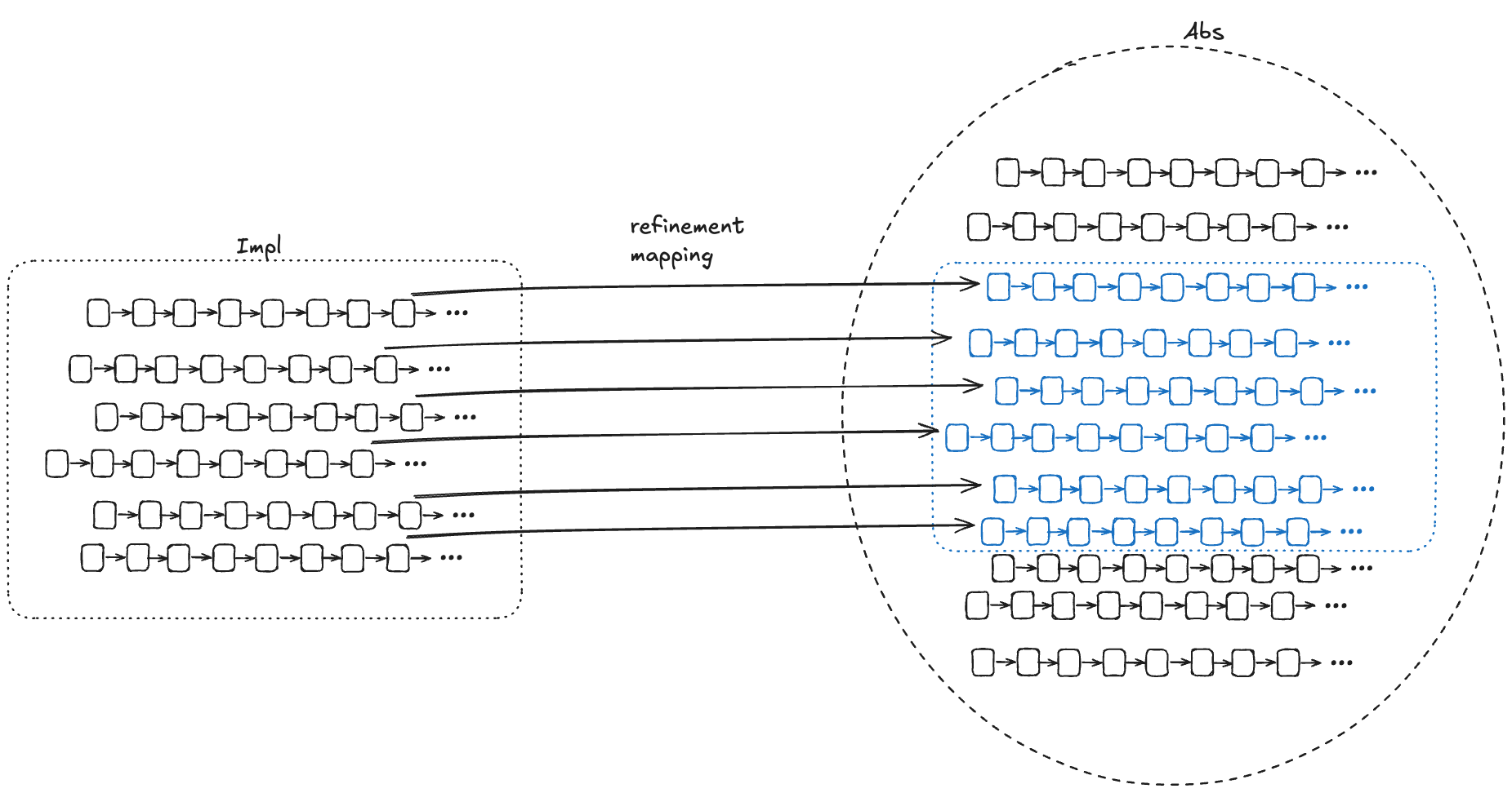
Checking serializability using refinement mapping
Just like we did previously with MVCC, we can define a refinement mapping from our SSI spec to our Serializability spec. You can find it in the SSIRefinement module (source, pdf). It’s almost identical to the MVCCRefinement module (source, pdf), with some minor modifications to handle the new abort scenarios.
The main difference is that now the refinement mapping should actually hold, because SSI ensures serializability! I wasn’t able to find a counterexample when I ran the model checker against the refinement mapping, so that gave me some confidence in my model. Of course, that doesn’t prove that my implementation is correct. But it’s good enough for a learning exercise.
Coda: on extending TLA+ specifications
Serializable Snapshot Isolation provides us with a nice example of when we can extend an existing specification rather than create a new one from scratch.
Even so, it’s still a fair amount of work to extend an existing specification. I suspect it would have been less work to take a copy-paste-and-modify approach rather than extending it. Still, I found it a useful exercise in learning how to modify a specification by extending it.
In a previous blog post, I talked about how we can use TLA+ to specify the serializability isolation level. In this post, we’ll see how we can use TLA+ to describe multi-version concurrency control (MVCC), which is a strategy for implementing transaction isolation. Postgres and MySQL both use MVCC to implement their repeatable read isolation levels, as well as a host of other databases.
MVCC is described as an optimistic strategy because it doesn’t require the use of locks, which reduces overhead. However, as we’ll see, MVCC implementations aren’t capable of achieving serializability.
We use a similar scheme as we did previously for modeling the externally visible variables. The only difference now is that we are also going to model the “start transaction” operation:
Variable name
Description
op
the operation (start transaction, read, write, commit, abort), modeled as a single letter: {“s”, “r”, “w”, “c”, “a”} )
arg
the argument(s) to the operation
rval
the return value of the operation
tr
the transaction executing the operation
The constant sets
There are three constant sets in our model:
Obj – the set of objects (x, y,…)
Val – the set of values that the objects can take on (e.g., 0,1,2,…)
Tr – the set of transactions (T0, T1, T2, …)
I associate the initial state of the database with a previously committed transaction T0 so that I don’t have to treat the initial values of the database as a special case.
The multiversion database
In MVCC, there can be multiple versions of each object, meaning that it stores multiple values associated with each object. Each of these versions is also has information on which transaction created it.
I modeled the database in TLA+ as a variable named db, here is an invariant that shows the values that db can take on:
It’s a function that maps objects to a set of version records. Each version record is associated with a value and a transaction. Here’s an example of a valid value for db:
Example db where Obj={x,y}
Playing the home game with Postgres
Postgres’s behavior when you specify repeatable read isolation level appears to be consistent with the MVCC TLA+ model I wrote so I’ll use it to illustrate some how these implementation details play out. As Peter Alvaro and Kyle Kingsbury note in their Jepsen analysis of MySQL 8.0.34, Postgres’s repeatable read isolation level actually implements snapshot isolation, while MySQL’s repeatable read isolation level actually implements …. um … well, I suggest you read the analysis.
I created a Postgres database named tla. Because Postgres defaults to read committed, I changed the default to repeatable read on my database so that it would behave more like my model.
ALTER DATABASE tla SET default_transaction_isolation TO 'repeatable read';

create table obj (
    k char(1) primary key,
    v int
);

insert into obj (k,v) values ('x', 0), ('y', 0);
Starting a transaction: id and visibility
In MVCC, each transaction gets assigned a unique id, and ids increase monotonically.
Transaction id: tid
I modeled this with a function tid that maps transactions to natural numbers. I use a special value called None for the transaction id for transactions who have not started yet.
When a transaction starts, I assign it an id by finding the largest transaction id assigned so far (mxid), and then adding 1. This isn’t efficient, but for a TLA+ spec it works quite nicely:
In Postgres, you can get the ID of the current transaction by using the pg_current_xact_id function. For examplle:
$ psql tla
psql (17.0 (Homebrew))
Type "help" for help.

tla=# begin;
BEGIN
tla=*# select pg_current_xact_id();
 pg_current_xact_id
--------------------
                822
(1 row)
Visible transactions: vis
We want each transaction to behave as if it is acting against a snapshot of the database from when the transaction started.
We can implement this in MVCC by identifying the set of transactions that have previously committed, and ensuring that our queries only read from writes done by these transactions.
I modeled this with a function called vis which maps each transaction to a set of other transactions. We also want our own writes to be visible, so we include the transaction being started in the set of visible transactions:
For each snapshot, Postgres tracks the set of committed transactions using three variables:
xmin – the lowest transaction id associated with an active transaction
xmax – (the highest transaction id associated with a committed transaction) + 1
xip_list – the list of active transactions whose ids are less than xmax
In Postgres, you can use the pg_current_snapshot function, which returns xmin:xmax:xip_list:
These three variables are sufficient to determine whether a particular version is visible. For more on the output of pg_current_snapshot, check out the Postgres operations cheat sheet wiki.
Performing reads
A transaction does a read using the Get(t, obj) operator. This operator retrieves the visible version with the largest transaction id:
Performing writes
Writes are straightforward, they simply add new versions to db. However, if a transaction did a previous write, that previous write has to be removed. Here’s part of the action that writes obj with value val for transaction t:
The lost update problem and how MVCC prevents it
Consider the following pair of transactions. They each write the same value and then commit.
A serializable execution history
This is a serializable history. It actually has two possible serializations: T1,T2 or T2,T1
Now let’s consider another history where each transaction does a read first.
A non-serializable execution history
This execution history isn’t serializable anymore. If you try to sequence these, the second read will read 2 where it should read 3 due to the previous write.
Serializability is violated: the read returns 2 instead of 3
This is referred to as the lost update problem.
Here’s a concrete example of the lost update problem. Imagine you’re using a record as a counter: you read the value, increment the result by one, and then write it back.
SELECT v FROM obj WHERE k='x';
-- returns 3
UPDATE obj set v=4 WHERE k='x';
Now imagine these two transactions run concurrently. If neither sees the other’s write, then one of these increments will be lost: you will have missed a count!
MVCC can guard against this by preventing two concurrent transactions from writing to the same object. If transaction T1 has written to a record in an active transaction, and T2 tries to write to the same record, then the database will block T2 until T1 either commits or aborts. If the first transaction commits, the database will abort the second transaction.
You can confirm this behavior in Postgres, where you’ll get an error if you try to write to a record that has previously been written to by a transaction that was active and then committed:
$ psql tla
psql (17.0 (Homebrew))
Type "help" for help.

tla=# begin;
BEGIN
tla=*# update obj set v=1 where k='x';
ERROR:  could not serialize access due to concurrent update
tla=!#
In our model, a write is implemented by two actions:
BeginWr(t, obj, val) – the initial write request
EndWr(t, obj, val) – the successful completion of the write
We do not allow the EndWr action to fire if:
There is an active transaction that has written to the same object (here we want to wait until the other transaction commits or aborts)
There is a commit to the same object by a concurrent transaction (here we want to abort)
We also have an action named AbortWr that aborts if a write conflict occurs.
Deadlock!
There’s one problem with the approach above where we block on a concurrent write: the risk of deadlock. Here’s what happens when we run our model with the TLC model checker:
Here’s a diagram of this execution history:
The problem is that T1 wrote x first and T2 wrote y first, and then T1 got blocked trying to write y and T2 got blocked trying to write x. (Note that even though T1 started to write y before T2, T2 completed the write first).
We can deal with this problem by detecting deadlocks and aborting the affected transactions when they happen. We can detect deadlock by creating a graph of dependencies between transactions (just like in the diagram above!) and then look for cycles:
Here TC stands for transitive closure, which is a useful relation when you want to find cycles. I used one of the transitive closure implementations in the TLA+ examples repo.
Top-level of the specification
Here’s a top-level view of the specification, you can find the full MVCC specification in the repo (source, pdf):
Note how reads and writes have begin/end pairs. In addition, a BeginWr can end in an AbortWr if there’s a conflict or deadlock as discussed earlier.
For liveness, we can use weak fairness to ensure that read/write operations complete, transactions start, and that deadlock is detected. But for commit and abort, we need strong fairness, because we can have infinite sequences of BeginRd/EndRd pairs or BeginWr/EndWr pairs and Commit and Abort are not enabled in the middle of reads or writes.
My MVCC spec isn’t serializable
Now that we have an MVCC spec, we can check to see if implements our Serializable spec. In order to do that check, we’ll need to do a refinement mapping from MVCC to Serializable.
One challenge is that the initial state of the Serializable specification establishes the fate of all of the transactions and what their environments are going to be in the future:
The Init state for the Serializable spec
Adding a delay to the Serializability spec
In our MVCC spec, we don’t know in advance if a transaction will commit or abort. We could use prophecy variables in our refinement mapping to predict these values, but I didn’t want to do that.
What I did instead was to create a new specification, SerializabilityD (source, pdf), that delays these predictions until the second step of the behavior:
I could then do a refinement mapping MVCC ⇒ SerializabilityD without having to use prophecy variables.
Verifying that SerializabilityD actually implements Serializability
Note that it’s straightforward to do the SerializabilityD ⇒ Serializability refinement mapping with prophecy variables. You can find it in SerializabilityDRefinement (source, pdf):
The MVCC ⇒ SerializabilityD mapping
The MVCC ⇒ SerializabilityD refinement mapping is in the MVCCRefinement spec (source, pdf).
The general strategy here is:
Execute MVCC until all of the transactions complete, keeping an execution history.
Use the results of the MVCC execution to populate the SerializabilityD variables
Step through the recorded MVCC execution history one operation at a time
The tricky part is step 2, because we need to find a serialization.
Attempting to find a serialization
Once we have an MVCC execution history, we can try to find a serialization. Here’s the relevant part of the SetFate action that attempts to select the to and benv variables from Serializability that will satisfy serializability:
Checking the refinement mapping
The problem with the refinement mapping is that we cannot always find a serialization. If we try to model check the refinement mapping, TLC will error because it is trying to CHOOSE from an empty set.
This MVCC execution history is a classic example of what’s called write skew. Here’s a visual depiction of this behavior:
A non-serializable execution history that is permitted by MVCC
Neither T1,T2 nor T2,t1 is a valid serialization of this execution history:
If we sequence T1 first, then the r[y,0] read violates the serialization. If we sequence T2 first, then the r[x,0] read violates it.
These constraints are what Adya calls anti-dependencies. He uses the abbreviation rw for short, because the dependency is created by a write from one transaction clobbering a read done by the other transaction, so the write has to be sequenced after the read.
Because snapshot isolation does not enforce anti-dependencies, it generates histories that are not serializable, which means that MVCC does not implement the Serializability spec.
Coda
I found this exercise very useful in learning more about how MVCC works. I had a hard time finding a good source to explain the concepts in enough detail for me to implement it, without having to read through actual implementations like Postgres, which has way too much detail. One useful resource I found was these slides on MVCC by Joy Arulraj at Georgia Tech. But even here, they didn’t have quite enough detail, and my model isn’t quite identical. But it was enough to help me get started.
I also enjoyed using refinement mapping to do validation. In the end, these were the refinement mappings I defined:
I’d encourage you to try out TLA+, but it really helps if you have some explicit system in mind you want to model. I’ve found it very useful for deepening my understanding of consistency models.
When I first learned about the mutual exclusion problem, it seemed easy and the published algorithms seemed needlessly complicated. So, I dashed off a simple algorithm and submitted it to CACM. I soon received a referee’s report pointing out the error. This had two effects. First, it made me mad enough at myself to sit down and come up with a real solution. The result was the bakery algorithm described in [12]. The second effect was to arouse my interest in verifying concurrent algorithms.
Modeling concurrency control in database systems is a great use case for TLA+, so I decided to learn use TLA+ to learn more about database isolation. This post is about modeling serializability.
You can find all of the the TLA+ models referenced in this post in my snapshot-isolation-tla repo. This post isn’t about snapshot isolation at all, so think of the name as a bit of foreshadowing of a future blog post, which we’ll discuss at the end.
Modeling a database for reasoning about transaction isolation
In relational databases, data is modeled as rows in different tables, where each table has a defined set of named columns, and there are foreign key relationships between the tables.
However, when modeling transaction isolation, we don’t need to worry about those details. For the purpose of a transaction, all we care about is if any of the columns of a particular row are read or modified. This means we can ignore details about tables, columns, and relations. All we care about are the rows.
The transaction isolation literature talks about objects instead of rows, and that’s the convention I’m going to use. Think of an object like a variable that is assigned a value, and that assignment can change over time. A SQL select statement is a read, and a SQL update statement is a write.
An example of how we’re modeling the database
Note that the set of objects is fixed during the lifetime of the model, it’s only the values that change over time. I’m only going to model reads and writes, but it’s simple enough to extend this model to support creation and deletion by writing a tombstone value to model deletion, and having a not-yet-created-stone value to model an object that has not yet been created in the database.
I’ll use the notation r[obj, val] to refer to a read operation where we read the object obj and get the value val and w[obj, val] to mean where we write the value val to obj. So, for example, setting x=1 would be: w[x, 1], and reading the value of x as 1 would be r[x, 1].
I’m going to use Obj to model the set of objects, and Val to model the set of possible values that objects can take on.
Obj is the set of objects, Val is the set of values that can be assigned to objects
We can model the values of the objects at any point in time as a function that maps objects to values. I’ll call these sorts of functions environments (env for short) since that’s what people who write interpreters call them.
Example of an environment
As an example of syntax, here’s how we would assert in TLA+ that the variable env is a function that maps element of the set Obj to elements of the set Val:
The execution of concurrent SQL-transactions at isolation level SERIALIZABLE is guaranteed to be serializable. A serializable execution is defined to be an execution of the operations of concurrently executing SQL-transactions that produces the same effect as some serial execution of those same SQL-transactions. A serial execution is one in which each SQL-transaction executes to completion before the next SQL-transaction begins.
An execution history of reads and writes is serializable if it is equivalent to some other execution history where the committed transactions are scheduled serially (i.e., they don’t overlap in time). Here’s an example of a serializable execution history.
It’s important to remember that a specification is just a set of behaviors (series of state transitions). We’re going to use TLA+ to define the set of all of the behaviors that we consider valid for serializability. Another way to put that is that our specification is the set of all serializable executions.
We want to make sure that if we build an implementation, all of the behaviors permitted by the implementation are a subset of our serializability specification.
Note: Causality is not required
Here’s an example of an execution history that is serializable according to the definition:
This looks weird to us because the write happens after the read: T1 is reading data from the future!
But the definition of serializability places no constraints on the ordering of the transaction, for that you need a different isolation level: strict serializability. But we’re modeling serializability, not strict serializability, so we allow histories like the one above in our specification.
(I’d say “good luck actually implementing a system that can read events from the future”, but in distributed databases when you’re receiving updates from different nodes at different times, some pretty weird stuff can happen…)
If you’d like to follow along as we go, my Serializable TLA+ model is in the github repo (source, pdf).
Externally visible variables
My specification will generate operations (e.g., reads, writes, commits, aborts). The four externally visible variables in the specification are:
Variable name
Description
op
the operation (read, write, commit, abort), modeled as a single letter: {“r”, “w”, “c”, “a”} )
arg
the argument(s) to the operation
rval
the return value of the operation
tr
the transaction executing the operation
Here’s the serializable example from earlier:
The execution history shown above can be modeled as a TLA+ behavior like this:
Initial state of the specification
We need to specify the set of valid initial states. In the initial state of our spec, before any operations are issued, we determine:
which transactions will commit and which will abort
the order in which the transactions will occur
the value of the environment for each committed transaction at the beginning and at the end of its lifetime
This is determined by using three internal variables whose values are set in the initial state:
Variable
Description
fate
function which encodes which transactions commit and which abort
to
transaction order
benv
the value of the environments at the beginning/end of each transaction
We couldn’t actually implement a system that could predict in advance whether a transaction will commit or abort, but it’s perfectly fine to use these for defining our specification.
The values of these variables are specified like this:
In our initial state, our specification chooses a fate, ordering, and begin/end environments for each transaction. Where Orderings is a helper operator:
As an example, consider a behavior with three transactions fated to commit, where the fated transaction order is:
T2
T3
T1
Furthermore, assume the following starting environments for each transaction:
T1: [x=2, y=5, z=3] T2: [x=0, y=0, z=0] T3: [x=0, y=1, z=0] Finally, assume that the final environment state (once T1 completes) is [x=2,y=5,z=1].
We can visually depict the committed transactions like like this:
Reads and writes
You can imagine each transaction running in parallel. As long as each transaction’s behavior is consistent with its initial environment, and it ends up with its final environment the resulting behavior will be serializable. Here’s an example.
Each transaction has a local environment, tenv. If the transaction is fated to commit, its tenv is initialized to its benv at the beginning:
where:
Here’s an example that shows how tenv for transaction T3 varies over time:
benv is fixed, but tenv for each transaction varies over time based on the writes
If the transaction is fated to abort, then we don’t track its environment in tenv, since any read or write is valid.
A valid behavior, as the definition of serializability places no constraints on the reads of an aborted transaction
Actions permitted by the specification
The specification permits the following actions:
commit transaction
abort transaction
read a value
write a value
I’m not modeling the start of a transaction, because it’s not relevant to the definition of serializability. We just assume that all of the transactions have already started.
In TLA+, we specify it like this:
Note that there are no restrictions here on the order in which operations happen. Even if the transaction order is [T2, T3, T1], that doesn’t require that the operations from T2 have to be issued before the other two transactions.
Rather, the only constraints for each transaction that will commit is that:
Its reads must be consistent with its initial environment, as specified by benv.
Its local environment must match the benv of the next transaction in the order when it finally commits.
We enforce (1) in our specification by using a transaction-level environment, tenv, for the reads. This environment gets initialized to benv for each transaction, and is updated if the transaction does any writes. This enables each transaction to see its own writes.
We enforce (2) by setting a precondition on the Commit action that it can only fire when tenv for that transaction is equal to benv of the next transaction:
Termination
If all of the transactions have committed or aborted, then the behavior is complete, which is modeled by the Termination sub-action, which just keeps firing and doesn’t change any of the variables:
Liveness
In our specification, we want to ensure that every behavior eventually satisfies the Termination action. This means that all transactions either eventually commit or abort in every valid behavior of the spec. In TLA+, we can describe this desired property like this:
The diamond is a temporal operator that means “eventually”.
To achieve this property, we need to specify a liveness condition in our specification. This is a condition of the type “something we want to happen eventually happens”.
We don’t want our transactions to stay open forever.
For transactions that are fated to abort, they must eventually abort
For transactions that are fated to commit, they must eventually commit
We’re going to use weak and strong fairness to specify our liveness conditions; for more details on liveness and fairness, see my post a liveness example in TLA+.
Liveness for aborts
We want to specify that everyone transaction that is fated to abort eventually aborts. To do this, we can use weak fairness.
This says that “the Abort action cannot be forever enabled without the Abort action happening”.
Here’s the Abort action.
The abort action is enabled for a transaction t if the transaction is in the open state, and its fate is Aborted.
Liveness for commits
The liveness condition for commit is more subtle. A transaction can only commit if its local environment (tenv) matches the starting environment of the transaction that follows it in transaction order (benv).
Consider two scenarios: one where tenv matches the next benv, and one where it doesn’t:
We want to use fairness to specify that every transaction fated to commit eventually reaches the state of scenario 1 above. Note that scenario 2 is a valid state in a behavior, it’s just not a state from which a commit can happen.
Consider the following diagram:
For every value of tenv[Ti], the number of variables that match the values in benv[i+1] is somewhere between 0 and 5. In the example above, there are two variables that match, x and z.
Note that the Commit action is always enabled when a transaction is open, so with every step of the specification, tenv can move left or right in the diagram above, with a min of 0 and a max of 5.
We need to specify “tenv always eventually moves to the right”. When tenv is at zero, we can use weak fairness to specify that it eventually moves from 0 to 1.
To specify this, I defined a function W(0, 1) which is true when tenv moves from 0 to 1:
Where M(env1, env2) is a count of the number of variables that have the same value:
This means we can specify “tenv cannot forever stay at 0” using weak fairness, like this:
We also want to specify that tenv eventually moves from 1 matches to 2, and then from 2 to 3, and so on, all of the way from 4 to all 5. And then we also want to say that it eventually goes from all matches to commit.
We can’t use weak fairness for this, because if tenv is at 1, it can also change to 0. However, the weak fairness of W(0,1) ensures that it if it goes from 1 down to 0, it will always eventually go back to 1.
Instead, we need to use strong fairness, which says that “if the action is enabled infinitely often, then the action must be taken”. We can specify strong fairness for each of the steps like this:
Recall that Obj is the set of objects {x, y, z, …}, and Cardinality refres to the size of the set. We also need to specify strong fairness on the commit action, to ensure that we eventually commit if all variables matching is enabled infinitely often:
Now putting it all together, here’s one way to specify the liveness condition, which is conventionally called L.
Once again, the complete model is in the github repo (source, pdf).
How do we know our spec is correct?
We can validate our serializable specification by creating a refinement mapping to a sequential specification. Here’s a simple sequential specification for a key-value store, Sequential.tla:
I’m not going to get into the details of the refinement mapping in this post, but you can find it at in the SerializabilityRefinement model (source, pdf).
OK, but how do you know that this spec is correct?
It’s turtles all of the way down! This is really the bottom in terms of refinement, I can’t think of an even simpler spec that we can use to validate this one.
However, one thing we can do is specify invariants that we can use to validate the specification, either with the model checker or by proof.
For example, here’s an invariant that checks whether each write has an associated read that happened before:
where:
But what happens if there’s no initial write? In that case, we don’t know what the read should be. But we do know that we don’t want to allow two successive reads to read different values, for example:
r[x,3], r[x,4]
So we can also specify this check as an invariant. I called that SuccessiveReads, you can find it in the MCSequential model (source, pdf).
The value of formalizing the specification
Now that we have a specification for Serializability, we can use it to check if a potential concurrency control implementation actually satisfies this specification.
That was my original plan for this blog post, but it got so long that I’m going to save that for a future blog post. In that future post, I’m going to model multi-version concurrency control (MVCC) and show how it fails to satisfy our serializability spec by having the model checker find a counterexample.
However, in my opinion, the advantage of formalizing a specification is that it forces you to think deeply about what it is that you’re specifying. Finding counter-examples with the model checker is neat, but the real value is the deeper understanding you’ll get.
If you’ve ever sat at a stop light that was just stuck on red, where there was clearly a problem with the light where it wasn’t ever switching green, you’ve encountered a liveness problem with a system.
Is the turning light just taking a long time? Or is it broken?
A liveness property of a specification is an assertion that some good thing eventually happens. In the case above, the something good is the light changing from red to green. If the light never turns green, then the system’s behavior violates the liveness property.
On the other hand, a safety property is an assertion that some bad thing never happens. To continue with the stop light example, you never want both the north-south and east-west traffic lights to be green at the same time. If those lights are both ever green simultaneously, then the system’s behavior violates the safety property. But this post is about liveness, not safety.
I’m going to walk through a simple TLA+ example that demonstrates why and how to specify liveness properties. Instead of using stop lights as my example, I’m going to use elevators.
A simple elevator specification
I’m going to build a minimalist TLA+ model of an elevator system. I’m going to model a building with N floors, and a single elevator, where the elevator is always either:
at a floor
between two floors
To keep things very simple, I’m not going to model things like passengers, doors, or call buttons. I’m just going to assume the elevator moves up and down in the building on its own.
To start with, the only constraint I’m going to put on the way the elevator moves is that it can’t change directions when it’s between two floors. For example, if the elevator is on floor 2, and then starts moving up, and is between floors 2 and 3, it can’t change direction and go back to floor 2: it has to continue on to floor 3. Once it’s on floor 3, it can go up or down. (Note: this is an example of a safety property).
My model is going to have two variables:
i – a natural number between 1 and 2×(# of floors) – 1
dir – the direction that the elevator is moving in (Up or Dn)
Assume we are modeling a building with 3 floors, then i would range from 1 to 5, and here’s how we would determine the floor that the elevator was on based on i.
i
floor
1
1
2
between 1 and 2
3
2
4
between 2 and 3
5
3
Note that when i is odd, the elevator is at a floor, and when even, the elevator is between floors. I use a hyphen (-) to indicate when the elevator is between floors.
Here’s a TLA+ specification that describes how this elevator moves. The spec permits four actions:
UpFlr – move up when at a floor
UpBetween – move up when between floors
DnFlr – move down when at a floor
DnBetween – move down when between floors
---- MODULE elevator ----
EXTENDS Naturals

CONSTANTS N, Up, Dn
ASSUME N \in Nat

VARIABLES i, dir

(* True when elevator is at floor f *)
At(f) == i+1 = 2*f

(* True when elevator is between floors *)
IsBetween == i % 2 = 0

Init == /\ i = 1
        /\ dir \in {Up, Dn}

(* move up when at a floor *)
UpFlr == /\ \E f \in 1..N-1 : At(f)
         /\ i' = i + 1
         /\ dir' = Up

(* move up when between floors *)
UpBetween == /\ IsBetween
             /\ dir = Up
             /\ i' = i + 1
             /\ UNCHANGED dir

(* move down when at a floor *)
DnFlr == /\ \E f \in 2..N : At(f)
         /\ i' = i-1
         /\ dir' = Dn

(* move down when between floors *)
DnBetween == /\ IsBetween
             /\ dir = Dn
             /\ i' = i - 1
             /\ UNCHANGED dir

Next == \/ UpFlr
        \/ UpBetween
        \/ DnFlr
        \/ DnBetween

v == <<i, dir>>
Spec == Init /\ [][Next]_v

====
Avoiding getting stuck
We don’t want the elevator to get stuck forever between two floors.
We’re trying to avoid this happening forever
Getting stuck is an example of a liveness condition. It’s fine for the elevator to sometimes be in the state i=2. we just want to ensure that it never stays in that state forever.
We can express this desired property using temporal logic. I’m going to use the diamond <> operator, which means “eventually”, and the box [] operator, which means “always”. Here’s how I expressed the desired property that the elevator doesn’t get stuck:
In English, GetsStuckBetweenFloors states: eventually, the elevator is always between floors. And then we define DoesntGetsStuckBetweenFloors as the negation of that.
We can check this property in the TLC model checker, by specifying it as a property in the config file:
PROPERTY
    DoesntGetsStuckBetweenFloors
If we check this with the spec from above, the model checker will find a behavior that is permitted by our specification, but that violates this property.
The behavior looks like this, floor: [1, -, -, -, …]. The elevator moves up between floors and then gets stuck there, exactly what we don’t want to happen.
Our specification as initially written does not prevent this kind of behavior. We need to add additional constraints to our specification so that the spec does not permit behaviors where the elevator gets stuck forever.
Specifying liveness with fairness properties
One thing we could do is simply conjoin the DoesntGetsStuckBetweenFloors property to our specification.
Spec == Init /\ [][Next]_v /\ ~<>[]IsBetween
This would achieve the desired effect, our spec would no longer permit behaviors where the elevator gets stuck between floors.
The problem with adding liveness constraints by adding an arbitrary temporal property to your spec is that you can end up unintentionally adding additional safety constraints to your spec. That makes your spec harder to reason about. Lamport provides a detailed example of how this can happen in chapter 4 of his book A Science of Concurrent Programs.
Conjoining arbitrary temporal logic expressions to your specification to specify liveness properties makes Leslie Lamport sad
In order to make it easier for a human to reason about a specification, we always want to keep our safety properties and our liveness properties separate. This means that when we add liveness properties to our spec, we want to guarantee that we don’t do it in such a way that we end up adding new safety properties as well.
We can ensure that we don’t accidentally sneak in any new safety properties by using what are called fairness properties to achieves our desired liveness property.
Using weak fairness to avoid getting stuck
Weak fairness of an action says that if the action A is forever enabled, then eventually there is an A step. That’s not a very intuitive concept, so I find the contrapositive more useful: If weak fairness of action A is true, then it cannot be that the system gets “stuck” forever in a state where it could take an A step, but doesn’t.
In TLA+, we specify weak fairness of an action like this:
WF_v(A)
This means that it can’t happen that A eventually becomes forever enabled without eventually taking an A step, where the A step changes the variable expression v (that means v’ has to be different from v).
We have two actions that fire when the elevator is between floors: UpBetween (when it’s between floors, going up), and DnBetween (when it’s between floors going down).
We can define our liveness condition like this:
L == WF_v(UpBetween) /\ WF_v(DnBetween)

Spec == Init /\ [][Next]_v /\ L
This says that if the model cannot be in a state forever where UpBetween is enabled but the UpBetween action never happens, and similarly for DnBetween.
And now the model checker returns success!
Visiting every floor
In our specification, we’d also like to guarantee that the elevator always eventually visits every floor, so that nobody is ever eternally stranded waiting for an elevator to arrive.
Here’s how I wrote this property: it’s always that true that, for every floor, the elevator eventually visits that floor:
VisitsEveryFloor == [] \A f \in 1..N : <>At(f)
If we check this property against our spec with TLC, it quickly finds a counterexample, the scenario where the elevator just sits on the ground floor forever! It looks like this: floor [1, 1, 1, 1, 1, ….]
We previously added weak fairness constraints for when the elevator is between floors. We can add additional fairness constraints so that the elevator can’t get stuck on any floors, that if it can move up or down, it has to eventually do so. Our liveness condition would look like this:
L == /\ WF_v(UpBetween)
     /\ WF_v(DnBetween)
     /\ WF_v(UpFlr)
     /\ WF_v(DnFlr)
But adding these fairness conditions don’t satisfy the VisitsEveryFloor property either! Here’s the counterexample:
In this counter-example, the behavior looks like this: floor [1, -, 2, -, 1, -, 2, -, …]. The elevator is cycling back and forth between floor 1 and floor 2. In particular, it never goes up past floor 2. We need to specify fairness conditions to prohibit a behavior like this.
Weak fairness doesn’t work here because the problem isn’t that the elevator is getting stuck forever on floor 2. Instead, it’s forever going back and forth between floors 1 and 2.
The elevator isn’t getting stuck, but it also is never going to floor 3
There’s a different fairness property, called strong fairness, which is similar to weak fairness, except that it also applies not just if the system gets stuck forever in a state, but also if a system goes in and out of that state, as long as it enters that state “infinitely often”. Basically, if it toggles forever in and out of that state, then you can use strong fairness to enforce an action in that state.
Which is exactly what the case is with our elevator, we want to assert that if the elevator reaches floor 2 infinitely often, it should eventually keep going up. We could express that using strong fairness like this:
SF_v(UpFlr /\ At(2))
Except that we don’t want this fairness condition to only apply at floor 2: we want it to apply for every floor (except the top floor). We can write it like this:
\A f \in 1..N-1: SF_v(UpFlr /\ At(f))
If we run the model checker again (where N=3), it still finds a counter-example(!):
Now the elevator does this: [1, -, 2, -, 3, 3, 3, 3, …]. It goes to the top floor and just stays there. It hits every floor once, but that’s not good enough for us: we want it to always eventually hit every floor.
We need to add some additional fairness conditions so that it the elevator also always eventually goes back down. Our liveness condition now looks like this:
L == /\ WF_v(UpBetween)
     /\ WF_v(DnBetween)
     /\ \A f \in 1..N-1: SF_v(UpFlr /\ At(f))
     /\ \A f \in 2..N: SF_v(DnFlr /\ At(f))
And this works!
Weak fairness on UpFlr and DnFlr is actually sufficient to prevent the elevators from getting stuck at the bottom or top floor, but we need strong fairness in the middle floors to ensure that the elevators always eventually visit every single floor.
Why can’t we just specify strong fairness of the UpFlr and DnFlr actions?
L == /\ WF_v(UpBetween)
     /\ WF_v(DnBetween)
     /\ SF_v(UpFlr)
     /\ SF_v(DnFlr)
The model checker can provide us with a counterexample to help explain why this liveness property doesn’t guarantee that the elevator always eventually visits all floors:
Here’s the pattern: [1,-,2,-,1,-,2,-,1,…]. We saw this behavior earlier, where the elevator just moves back and forth between floor 1 and floor 2.
The problem is that both SF_v(UpFlr) and SF_v(DnFlr) are satisfied by this behavior, because the elevator always eventually goes up (from floor 1) and always eventually goes down (from floor 2).
If we want the elevator to eventually visit every floor, then we need to specify the fairness conditions separately for each floor.
Further reading
Hillel Wayne’s blog posts are always a great introduction to TLA+ concepts:
Justine Tunney recently wrote a blog post titled The Fastest Mutexes where she describes how she implemented mutexes in Cosmopolitan Libc. The post discusses how her implementation uses futexes by way of Mike Burrows’s nsync library. From her post
nsync enlists the help of the operating system by using futexes. This is a great abstraction invented by Linux some years ago, that quickly found its way into other OSes. On MacOS, futexes are called ulock. On Windows, futexes are called WaitOnAddress(). The only OS Cosmo supports that doesn’t have futexes is NetBSD, which implements POSIX semaphores in kernelspace, and each semaphore sadly requires creating a new file descriptor. But the important thing about futexes and semaphores is they allow the OS to put a thread to sleep. That’s what lets nsync avoid consuming CPU time when there’s nothing to do.
Before I read this post, I had no idea what futexes were or how they worked. I figured a good way to learn would be to model them in TLA+.
Note: I’m going to give a simplified account of how futexes work. In addition, I’m not an expert on this topic. In particular, I’m not a kernel programmer, so there may be important details I get wrong here.
Mutexes
Readers who have done multithreaded programming before are undoubtedly familiar with mutexes: they are a type of lock that allows the programmer to enforce mutual exclusion, so that we can guarantee that at most one thread accesses a resource, such as a shared variable.
The locking mechanism is implemented by the operating system: locking and unlock the mutex ultimately involves a system call. If you were programming in C on a Unix-y system like Linux, you’d use the pthreads API to access the mutex objects. Which pthreads implementation you use (e.g., glibc, musl) will make the relevant system calls for you.
#include <pthread.h>
...
// create a mutex
pthread_mutex_t mutex = PTHREAD_MUTEX_INITIALIZER;

pthread_mutex_lock(&mutex);
// mutex is now locked

pthread_mutex_unlock(&mutex);
// mutex is now unlocked
Modeling a mutex in TLA+
Before we get into futexes, let’s start off by modeling desired behavior of a mutex in TLA+. I’ll use the PlusCal algorithm language for my model, which can be translated directly to a TLA+ model (see my mutex.tla file)
This model defines a fixed set of Processes. You should really think of these as threads, but there’s a convention in academia to refer to them as processes, so I used that convention. You can think of Processes in this model as a set of threads ids.
Modeling the lock
This model has only explicit variable, named lock, which is my model for the mutex lock. I’ve modeled it as a set. When the lock is free, the set is empty, and when the lock is held by a process, the set contains a single element, the process id.
Process states
PlusCal models also have an implicit variable, pc for program counter. The program counter indicates which state each process is in.
Each process can be in one of four states. We need to give a label to each of these states in our model.
Label
Description
ncs
in the non-critical section (lock is not held)
acq
waiting to acquire the lock
cs
in the critical section (lock is held)
rel
releasing the lock
We want to make sure that two processes are never in the critical section at the same time. We can express this desired property in TLA+ like this:
We can specify MutualExclusion as an invariant and use the TLC model checker to verify that our specification satisfies this property. Check out mutex.cfg for how to configure TLC to check the invariant.
Overhead of traditional mutexes
With a traditional mutex, the application make a system call every time the mutex is locked or unlocked. If the common usage pattern for an application is that there’s only one thread that tries to take the mutex, then you’re paying a performance penalty for having to execute those system calls. If the mutex is being acquired and released in a tight loop, then the time that goes to servicing the system calls could presumably be a substantial fraction of the execution time of the loop.
for(...) {
  pthread_mutex_lock(&mutex);
  // do work here
  pthread_mutex_unlock(&mutex);
}
I don’t know how high these overheads are in practice, but Justine Tunney provides some numbers in her blog post as well as a link to Mark Waterman’s mutex shootout with more performance numbers.
Ideally, we would only pay the performance penalty for system calls when the mutex was under contention, when there were multiple threads that were trying to acquire the lock.
Futexes: avoid the syscalls where possible
Futexes provide a mechanism for avoiding system calls for taking a mutex lock in cases where the lock is not under contention.
More specifically, futexes provide a set of low-level synchronization primitives. These primitives allow library authors to implement mutexes in such a way that they avoid making system calls when possible. Application programmers don’t interact with futexes directly, they’re hidden behind APIs like pthread_mutex_lock.
Primitives: wait and wake
The primary two futex primitives are a wait system call and a wake system call. Each of them take an integer pointer as an argument, which I call futex. Here’s a simplified C function prototype for each of them.
(Actual versions of these return status codes, but I won’t be using those return codes in this blog post).
Note that the futex_wait prototype shown above is incomplete: it needs to take an additional argument to guarantee correctness, but we’ll get to that later. I want to start off by providing some intuition on how to use futexes.
When a thread calls the futex_wait system call, the kernel puts the thread to sleep until another thread calls futex_wake with the same futex argument.
Using primitives to build mutexes that avoid system calls
OK, so how do we actually use these things to create mutexes?
Here’s a naive (i.e., incorrect) implementation of lock and unlock functions that implement mutual exclusion using the futex calls. The lock function checks if the lock is free. If it is, it takes the lock, otherwise it waits to be woken up and then tries again.
#define FREE 0
#define ACQUIRED 1
#define CONTENDED 2
void futex_wait(int *futex);
void futex_wake(int *futex);
/**
* Try to acquire the lock. On failure, wait and then try again.
*/
void lock(int *futex) {
bool acquired = false;
while (!acquired) {
if (*futex == FREE) {
*futex = ACQUIRED;
acquired = true;
}
else {
*futex = CONTENDED;
futex_wait(futex, CONTENDED);
}
}
}
/**
* Release lock, wake threads that are waiting on lock
*/
void unlock(int *futex) {
int prev = *futex;
*futex = FREE;
if(prev == CONTENDED) {
futex_wake(futex);
}
}
Note that futex is just an ordinary pointer. In the fast path, the lock function just sets the futex to ACQUIRED, no system call is necessary. It’s only when the futex is not free that it has to make the futex_wait system call.
Similarly, on the unlock side, it’s only when the futex is in the CONTENDED state that the futex_wake system call happens.
Now’s a good time to point out that futex is short for fast userspace mutex. The reason it’s fast is because we can (sometimes) avoid system calls. And the reason we are able to avoid system calls is that, in the fast path, the threads coordinate by modifying a memory location that is accessible in userspace. By userspace, we mean that our futex variable is just an ordinary pointer that the threads all have direct access to: no system call is required to modify it.
By contrast, when we call futex_wait and futex_wake, the kernel needs to read and modify kernel data structures, hence a system call is required.
The code above should provide you with an intuition of how futexes are supposed to work. The tricky part is writing the algorithm in such a way as to guarantee correctness for all possible thread schedules. There’s a reason that Ulrich Drepper wrote a paper titled Futexes are Tricky: it’s easy to get the lock/unlock methods wrong.
Why futex_wait needs another agument
There are many potential race conditions in our initial lock/unlock implementation, but let’s focus on one in particular: if the futex gets freed after the lock checks if it’s free, but before calling futex_wait.
Here’s what the scenario looks like (think of the red arrows as being like breakpoints):
We need to prevent the situation where the unlock thread completes after the *futex == FREE check but before the futex_wait system call.
We can prevent this by modifying the futex_wait function prototype to pass the value we expect the futex to have, it looks like this:
void futex_wait(int *futex, int val);
The lock code then looks like this instead:
void lock(int *futex) {
    if(*futex == FREE) {
        *futex = ACQUIRED;
    } else {
        *futex = CONTENDED;
        futex_wait(futex, CONTENDED);
        // try again after waking up
        lock(futex);
    }
}
The futex_wait system call will check to ensure that *futex == val. So, if the *futex gets changed, the function will return immediately rather than sleeping.
Here’s the FUTEX_WAIT section of the Linux futex man page, which hopefully should be clear now.
FUTEX_WAIT (since Linux 2.6.0) This operation tests that the value at the futex word pointed to by the address uaddr still contains the expected value val, and if so, then sleeps waiting for a FUTEX_WAKE operation on the futex word. The load of the value of the futex word is an atomic memory access (i.e., using atomic machine instructions of the respective architecture). This load, the comparison with the expected value, and starting to sleep are performed atomically and totally ordered with respect to other futex operations on the same futex word. If the thread starts to sleep, it is considered a waiter on this futex word. If the futex value does not match val, then the call fails immediately with the error EAGAIN.
Atomic operations
In order for the lock/unlock implementations to guarantee correctness, we need to rely on what are called atomic operations when reading and modifying the futex across multiple threads. These are operations that the hardware guarantees can be performed atomically, so that there are no possible race conditions.
In my futex model, I assumed the existence of three atomic operations:
atomic store
atomic exchange
atomic compare and exchange
Atomic store isn’t very interesting, it just says that we can atomically set the value of a variable, i.e., that when we do something like this, it happens atomically.
*futex = FREE
In PlusCal, atomic stores are just modeled as assigning a value to a variable, so there’s not much else to sta
Atomic exchange
Atomic exchange looks like this:
oldval = atomic_exchange(x, newval)
You give atomic exchange two arguments: a variable (x) you want to modify, and the new value (newval) you want it to have. The atomic_exchange function will atomically set x=newval and return the value x had before the assignment.
In PlusCal, I modeled it as a macro. Macros can’t return values, so we need to pass in oldval as an argument.
macro atomic_exchange(x, oldval, newval) begin
    oldval := x;
    x := newval;
end macro;
Then I can invoke it like this in my PlusCal model:
atomic_exchange(mem[a], uprev, Free);
And the resulting behavior is:
uprev := mem[a];
mem[a] := Free;
Atomic compare and exchange
Atomic compare and exchange is sometimes called test-and-set. It looks like this:
It’s similar to atomic exchange, except that it only performs the exchange if the variable x contains the value expecting. Basically, it’s an atomic version of this:
if (x == expecting)
  oldval = atomic_compare_exchange(x, newval)
else
  oldval = x
In my PlusCal model, I also implemented it as a macro:
macro atomic_compare_exchange(x, oldval, expecting, newval) begin
    oldval := x;
    if x = expecting then
        x := newval;
    end if;
end macro;
Futex modeling basics
Here are the basics constants and variables in my model:
CONSTANTS Processes, Addresses, Free, Acquired, Contended

(*--algorithm futex

variables
    mem = [x \in Addresses |-> Free],
    a \in Addresses,
    ...
In addition to modeling Processes, my futex model also models a set of memory address as Addresses. I also defined three constants: Free, Acquired, Contended which have the same role as FREE, ACQUIRED, and CONTENDED in the example C code above.
I model memory as a function (mem) that maps addresses to values, as well as a specific memory address (a). I use a as my futex.
At the top-level, the algorithm should look familiar, it’s basically the same as the mutex.tla one, except that it’s calling acquire_lock and release_lock procedures.
process proc \in Processes
begin
    ncs: skip;
    acq: call acquire_lock();
    cs:  skip;
    rel: call release_lock();
         goto ncs;
end process;
acquire_lock: implementing lock
I based my implementation of the lock on a simplified version of the one in Ulrich Drupper’s Futexes are Tricky paper.
Here’s the model for acquiring the lock. It doesn’t render particularly well in WordPress, so you may want to view the futex.tla file on GitHub directly.
procedure acquire_lock()
variable lprev;
begin
           \* Attempt to acquire the lock
Lcmpx1:    atomic_compare_exchange(mem[a], lprev, Free, Acquired);
Ltest:     while lprev # Free do
              \* Mark the lock as contended, assuming it's in the acquired state
Lcmpx2:       atomic_compare_exchange(mem[a], lprev, Acquired, Contended);
              if lprev # Free then
call_wait:        call futex_wait(a, Contended);
              end if;
              \* Attempt to acquire the lock again
Lcmpx3:       atomic_compare_exchange(mem[a], lprev, Free, Contended);
           end while;
            \* if we reach here, we have the lock
Lret:      return;
end procedure;
Note that we need three separate atomic_compare_exchange calls to implement this (each with different arguments!). Yipe!
release_lock: implementing unlock
The unlock implementation is much simpler. We just set the futex to Free and then wake the waiters.
procedure release_lock()
variable uprev;
begin
u_xch:  atomic_exchange(mem[a], uprev, Free);
u_wake: if uprev = Contended then
           call futex_wake(a);
        end if;
u_ret:  return;
end procedure;
Modeling the futex_wait/futex_wake calls
Finally, it’s not enough in our model to just invoke futex_wait and futex_wake, we need to model the behavior of these as well! I’ll say a little bit about the relevant kernel data structures in the Linux kernel and how I modeled them
Kernel data structures
The Linux kernel hashes futexes into buckets, and each of these bucket is associated with a futex_hash_bucket structure. For the purposes of our TLA+ model, the fields we care about are:
queue of threads (tasks) that are waiting on the futex
lock for protecting the structure
The kernel also uses a structure called a wake-queue (see here for more details) to keep a list of the tasks that have been selected to be woken up. I modeled this list of threads-to-be-woken as a set.
Here are the variables:
variables
...
    waitq = [x \in Addresses |-> <<>>], \* a map of addresses to wait queues
    qlock = {},  \* traditional mutex lock used by the kernel on the wait queue.
    wake = {}; \* processes that have been sent a signal to wake up
I made the following assumptions to simplify my model
every futex (address) is associated with one queue, rather than hashing and bucketing
I used a global lock instead of having a per-queue lock
futex_wait
Here’s the basic futex_wait algorithm (links go to Linux source code)
Note: I assume that calling schedule() inside of the kernel at this point has the effect of putting the thread to sleep, but as I said earlier, I’m not a kernel programmer so I’m not familiar with this code at all.
Here’s my PlusCal model:
procedure futex_wait(addr, val)
begin
wt_acq:       await qlock = {};
              qlock := {self};
wt_valcheck:  if val /= mem[addr] then
                qlock := {};
                return;
              end if;
              \* Add the process to the wait queue for this address
wt_enq:       waitq[addr] := Append(waitq[addr], self);
              qlock := {};
wt_wait:      await self \in wake;
              wake := wake \ {self};
              return;
end procedure;
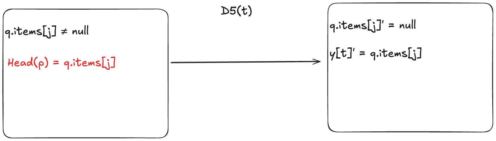
Here’s my PlusCal model of it. I chose to wake only one process in my model, but we could have have woken all of the waiting processes.
procedure futex_wake(addr)
variables nxt = {}
begin
wk_acq:   await qlock = {};
          qlock := {self};
wk_deq:   if waitq[addr] /= <<>> then
              nxt := {Head(waitq[addr])};
              waitq[addr] := Tail(waitq[addr]);
          end if;
wk_rel:   qlock := {};
wk_wake:  wake := wake \union nxt;
          return;
end procedure;
You can see the full model on GitHub at futex.tla.
Checking for properties
One of the reasons to model in TLA+ is to check properties of the specification. I care about three things with this specification:
It implements mutual exclusion
It doesn’t make system calls when there’s no contention
Processes can’t get stuck waiting on the queue forever
Mutual exclusion
We check mutual exclusion the same way we did in our mutex.tla specification, by asserting that there are never two different processes in the critical section at the same time. This is our invariant.
The whole point of using futexes to implement locks was to avoid system calls in the cases where there’s no contention. Even if our algorithm satisfies mutual exclusion, that doesn’t mean that it avoids these system calls.
I wrote an invariant for the futex_wait system call, that asserts that we only make the system call when there’s contention. I called the invariant OnlyWaitUnderContention, and here’s how I defined it. I created several helper definitions as well.
Recall earlier in the blog post how we had to modify the prototype of the futex_wait system call to take an additional argument, in order to prevent a race condition that could leave a process waiting forever on the queue.
We want to make sure that we have actually addressed that risk. Note that the comments in the Linux source code specifically call out this risk.
I checked this by defining an invariant that stated that it never can happen that a process is waiting and all of the other processes are past the point where they could wake up the waiter.
Stuck(x) == /\ pc[x] = "wt_wait"
            /\ x \notin wake
            /\ \A p \in Processes \ {x} : \/ pc[p] \in {"ncs", "u_ret"}
                                          \/ /\ pc[p] \in {"wk_rel", "wk_wake"}
                                             /\ x \notin nxt[p]

NoneStuck == ~ \E x \in Processes : Stuck(x)
Final check: refinement
In addition to checking mutual exclusion, we can check that our futex-based lock model (futex.tla) implements our original high-level mutex model (mutex.tla) by means of a refinement mapping.
To do that, we need to define mappings between the futex model variables and the mutex model variables. The mutex model has two variables:
lock – the model of the lock
pc – the program counters for the processes
I called my mappings lockBar and pcBar. Here’s what the mapping looks like:
We can then define a property that says that our futex specification implements the mutex specification:
ImplementsMutex == mutex!Spec
Finally, in our futex.cfg file, we can specify that we want to check the invariants, as well as this behavioral property. The relevant config lines look like this:
Back in August, Murat Derimbas published a blog post about the paper by Herlihy and Wing that first introduced the concept of linearizability. When we move from sequential programs to concurrent ones, we need to extend our concept of what “correct” means to account for the fact that operations from different threads can overlap in time. Linearizability is the strongest consistency model for single-object systems, which means that it’s the one that aligns closest to our intuitions. Other models are weaker and, hence, will permit anomalies that violate human intuition about how systems should behave.
Beyond introducing linearizability, one of the things that Herlihy and Wing do in this paper is provide an implementation of a linearizable queue whose correctness cannot be demonstrated using an approach known as refinement mapping. At the time the paper was published, it was believed that it was always possible to use refinement mapping to prove that one specification implemented another, and this paper motivated Leslie Lamport and Martín Abadi to propose the concept of prophecyvariables.
I have long been fascinated by the concept of prophecy variables, but when I learned about them, I still couldn’t figure out how to use them to prove that the queue implementation in the Herlihy and Wing paper is linearizable. (I even asked Leslie Lamport about it at the 2021 TLA+ conference).
Recently, Lamport published a book called The Science of Concurrent Programs that describes in detail how to use prophecy variables to do the refinement mapping for the queue in the Herlihy and Wing paper. Because the best way to learn something is to explain it, I wanted to write a blog post about this.
In this post, I’m going to assume that readers have no prior knowledge about TLA+ or linearizability. What I want to do here is provide the reader with some intuition about the important concepts, enough to interest people to read further. There’s a lot of conceptual ground to cover: to understand prophecy variables and why they’re needed for the queue implementation in the Herlihy and Wing paper requires an understanding of refinement mapping. Understanding refinement mapping requires understanding the state-machine model that TLA+ uses for modeling programs and systems. We’ll also need to cover what linearizability actually is.
We’ll going to start all of the way at the beginning: describing what it is that a program should do.
What does it mean for a program to be correct?
Think of an abstract data type (ADT) such as a stack, queue, or map. Each ADT defines a set of operations. For a stack, it’s push and pop , for a queue, it’s enqueue and dequeue, and for a map, it’s get, set, and delete.
Let’s focus on the queue, which will be a running example throughout this blog post, and is the ADT that is the primary example in the linearizability paper. Informally, we can say that dequeue returns the oldest enqueued value that has not been dequeued yet. It’s sometimes called a “FIFO” because it exhibits first-in-first-out behavior. But how do we describe this formally?
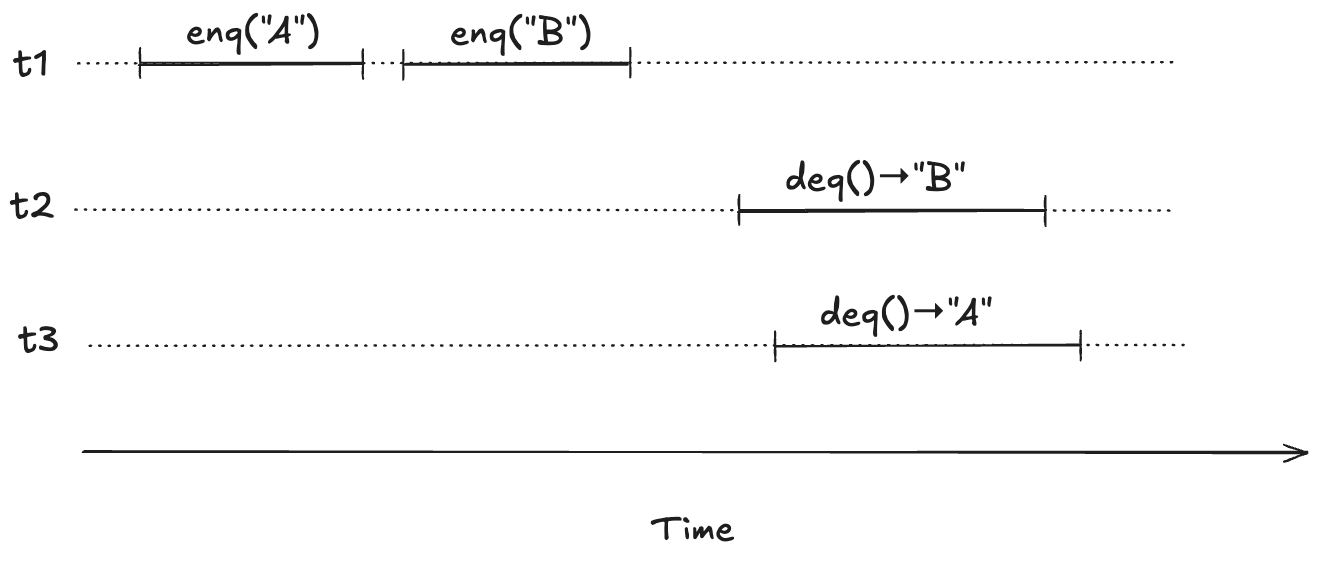
Think about how we would test that a given queue implementation behaves the way we expect. One approach is write a test that consists of a history of enqueue and dequeue operations, and check if our queue returns the expected values.
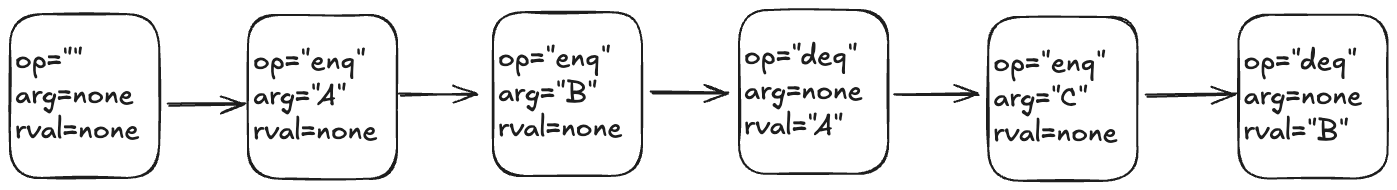
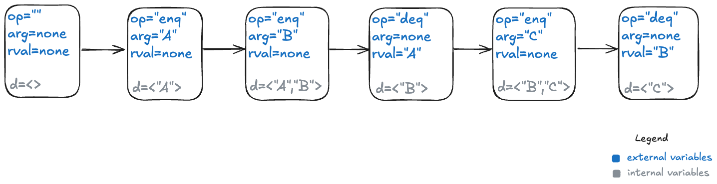
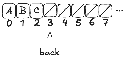
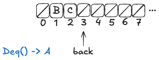
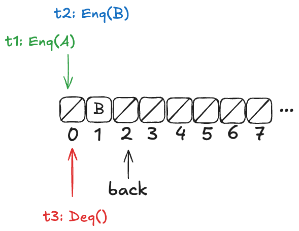
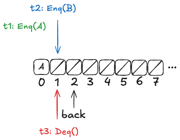
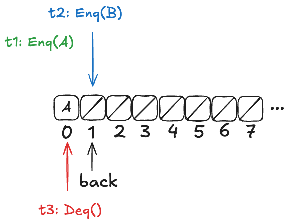
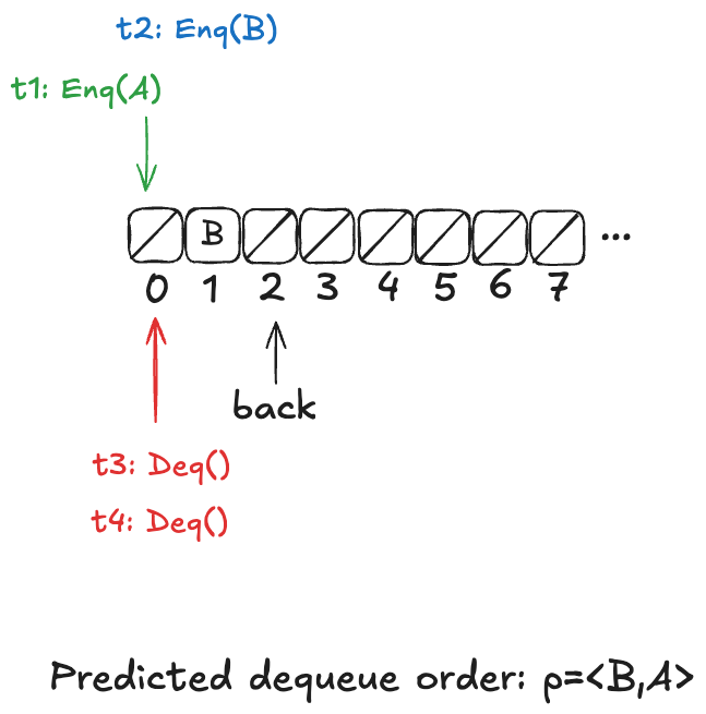
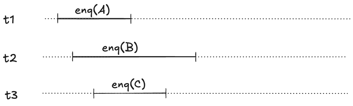
Here’s an example of an execution history, where enq is the enqueue operation and deq is the dequeue operation. Here I assume that enq does not return a value.
If we have a queue implementation, we can make these calls against our implementation and check that, at each step in the history, the operation returns the expected value, something like this:
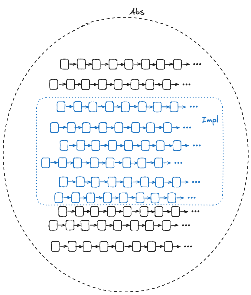
Of course, a single execution history is not sufficient to determine the correctness of our queue implementation. But we can describe the set of every possible valid execution history for a queue. The size of this set is infinite, so we can’t explicitly specify each history like we did above. But we can come up with a mathematical description of the set of every possible valid execution history, even though it’s an infinite set.
Specifying valid execution histories: the transition-axiom method
In order to specify how our system should behave, we need a way of describing all of its valid execution histories. We are particularly interested in a specification approach that works for concurrent and distributed systems, since those systems have historically proven to be notoriously difficult for humans to reason about.
In the 1980s, Leslie Lamport introduced a specification approach that he called the transition-axiom method. He later designed TLA+ as a language to support specifying systems using the transition-axiom method.
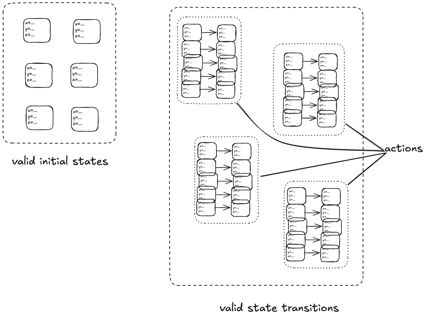
The transition-axiom method uses a state-machine model to describe a system. You describe a system by describing:
The set of valid initial states
The set of valid state transitions
(Aside: I’m not covering the more advanced topic of livenessin this post).
A set of related state transitions is referred to as an action. We use actions in TLA+ to model the events we care about (e.g., calling a function, sending a message).
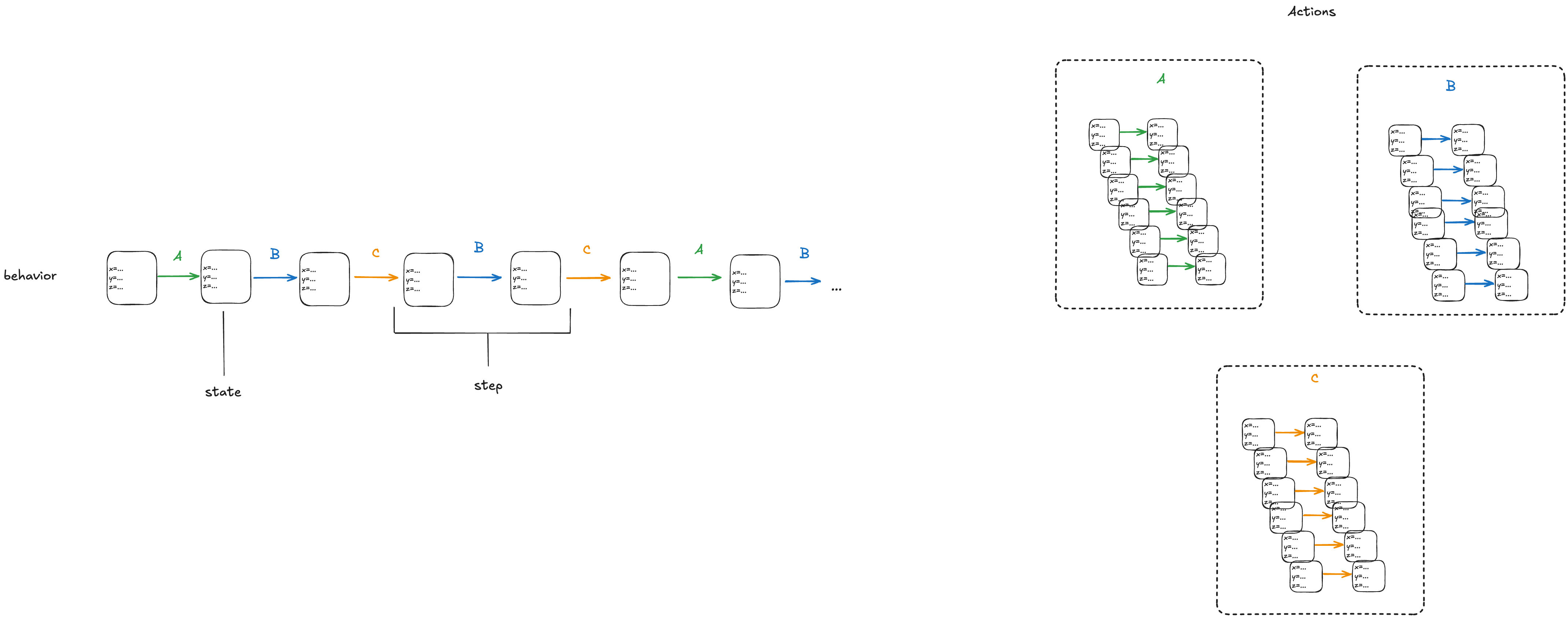
With a state-machine description, we can generate all sequences that start at one of the initial states and transition according to the allowed transitions. A sequence of states is called a behavior. A pair of successive states is called a step.
Each step in a behavior must be a member of one of the actions. In the diagram above, we would call the first step an A-step because it is a step that is a member of the A action.
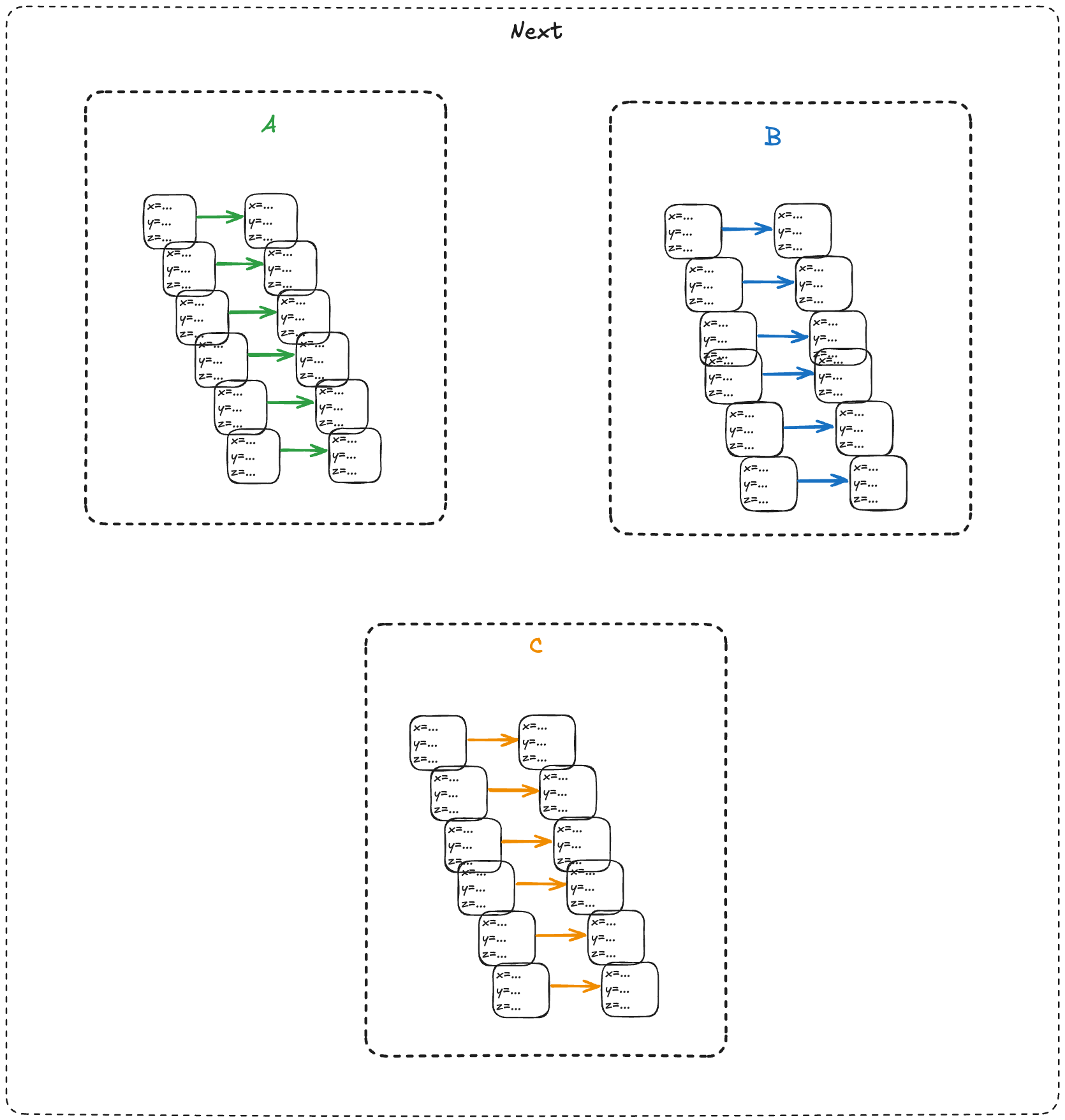
We refer to the set that includes all of the actions as the next-state action, which is typically called Next in TLA+ specifications.
In the example above, we would say that A, B, C are sub-actions of the Next action.
We call the entire state-machine description a specification: it defines the set of all allowed behaviors.
To make things concrete, let’s start with a simple example: a counter.
You think distributed systems is about trying to accomplish complex tasks, and then you read the literature and it's like "consider the problem of incrementing a counter", and it turns out that distributed systems is about how the simplest tasks become mind-bogglingly complex. https://t.co/4O2jfgfGQV
— @norootcause@hachyderm.io on mastodon (@norootcause) May 21, 2020
Modeling a counter with TLA+
Consider a counter abstract data type, that has only two operations:
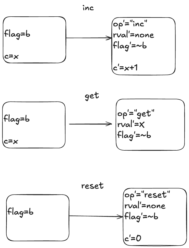
inc – increment the counter
get – return the current value of the counter
reset – return the value of the counter to zero
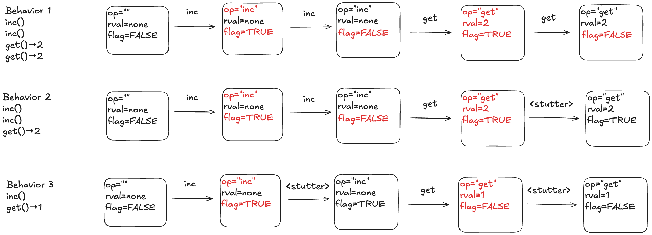
Here’s an example execution history.
inc()
inc()
get() → 2
get() → 2
reset()
get() → 0
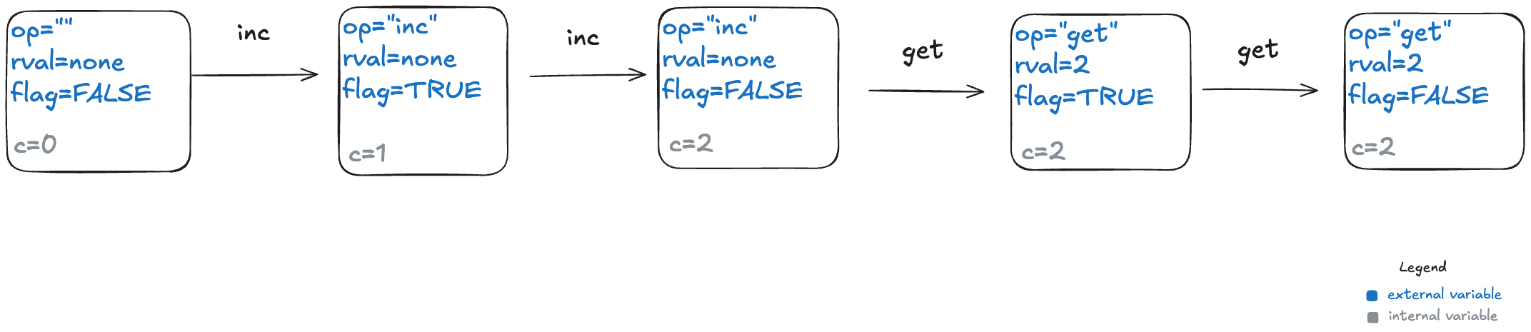
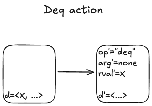
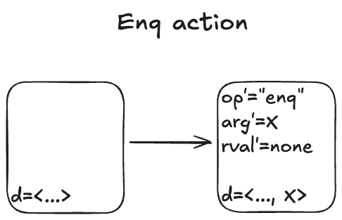
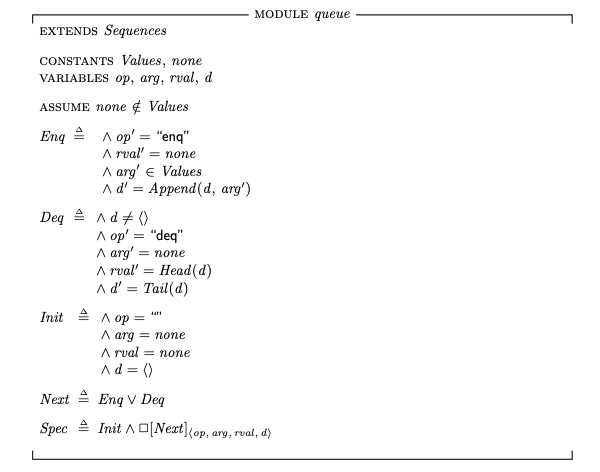
To model this counter in TLA+, we need to model the different operation types (inc, get, reset). We also need to model the return value for the get operation. I’ll model the operation with a state variable named op, and the return value with a state variable named rval.
But there’s one more thing we need to add to our model. In a state-machine model, we model an operation using one or more state transitions (steps) where at least one variable in the state changes. This is because all TLA+ models must allow what are called stuttering steps, where you have a state transition where none of the variables change.
This means we need to distinguish between two consecutive inc operations versus an inc operation followed by a stuttering step where nothing happens.
To do that, I’ll add a third variable to my model, which I’ll unimaginatively call flag. It’s a boolean variable, which I will toggle every time an operation happens. To sum up, my three state variables are:
op – the operation (“inc”, “get”, “reset”), which I’ll initialize to “” (empty string) in the first state
rval – the return value for a get operation. It will be a special value called none for all of the other operations
flag – a boolean that toggles on every (non-stuttering) state transition.
Below is a depiction of an execution history and how this would be modeled as a behavior at TLA+. The text in red indicated which variable changed in the transition. As mentioned above, every transition associated with an operation must have at least one variable that changes value.
Here’s a visual depiction of an execution history. Note how each event in the history is modeled as a step (pair of states) where at least one variable changes.
To illustrate why we need the extra variables, consider the following three behaviors.
In behavior 1, there are no stuttering steps. In behavior 2, the last step is a stuttering step, so there is only one “get” invocation. In behavior 3, there are two stuttering steps.
The internal variables
Our model of a counter so far has defined the external variables, which are the only variables that we really care about as the consumer of a specification. If you gave me a set of all of the valid behaviors for a queue, where behaviors were described using only these external behaviors, that’s all I need to understand how a queue behaves.
However, the external variables aren’t sufficient for the producer of a specification to actually generate the set of valid behaviors. This is because we need to keep track of some additional state information: how many increments there have been since the last reset. This type of variable is known as an internal state variable. I’m going to call this particular internal state variable c.
Here’s behavior 1, with different color codings for the external and internal variables.
The actions
Here is a visual depiction of the permitted state transitions. Recall the set of permitted state transitions is called an action. For our counter, there are three actions, which corresponds to the three different operations we model: inc, get, and reset.
Each transition is depicted as two boxes with variables in it. The left-hand box shows the values of the variables before the state transition, and the right-hand box shows the values of the variables after the state transition. By convention we add a prime (‘) to the variables to refer to their values after the state transition.
While the diagram depicts three actions, each action describes a set of allowed state transitions. As an example, here are two different state transitions that are both members of the inc set of permitted transitions.
[flag=TRUE, c=5] → [flag=FALSE, c=6]
[flag=TRUE, c=8]→ [flag=FALSE, c=9]
In TLA+ terminology, we call these two steps inc steps. Remember: in TLA+, all of the action is in the actions. We use actions (sets of permitted state transitions) to model the events that we care about.
Modeling a queue with TLA+
We’ll move on to our second example, which will form the basis for the rest of this post: a queue. A queue supports two operations, which I’ll call enq (for enqueue) and deq (for dequeue).
Modeling execution histories as behaviors
Recall our example of a valid execution history for a queue:
enq("A")
enq("B")
deq() → "A"
enq("C")
deq() → "B"
We now have to model argument passing, since the enq operation takes an argument.
Here’s one way to model this execution history as a TLA+ behavior.
My model uses three state variables:
op – identifies which operation is being invoked (enq or deq)
arg – the argument being passed in the case of the enq operation
rval – the return value in the case of the deq operatoin
TLA+ requires that we specify a value for every variable in every state, which means we need to specify a value for arg even for the deq operation, which doesn’t have an argument, and a value for rval for the enq operation, which doesn’t return a value. I defined a special value called none for this case.
In the first state, when the queue is empty, I chose to set op to the empty string (“”) and arg and rval to none.
The internal variables
For a queue, we need to keep track all of the values that have previously been enqueued, as well as the order in which they were enqueued.
TLA+ has a type called a sequence which I’ll use to encode this information: a sequence is like a list in Python.
I’ll add a new variable which I’ll unimaginatively call d, for data. Here’s what that behavior looks like with the internal variable.
Modeling dequeues
Recall that our queue supports two operations: enqueue and dequeue. We’ll start with the dequeue operation. I modeled it with an action called Deq.
Here are some examples of state transitions that are permitted by the Deq action. We call these Deq steps.
I’m not going to write much TLA+ code in this post, but to give you a feel for it, here is how you would write the Deq action in TLA+ syntax:
The syntax of the first line might be a bit confusing if you’re not familiar with TLA+:
# is TLA+ for ≠
<<>> is TLA+ for the empty sequence.
Modeling dequeues
Here’s what the Enq action looks like:
There’s non-determinism in this action: the value of arg’ can be any valid value that we are allowed to put onto the queue.
I’ll spend just a little time in this section to give you a sense of how you would use TLA+ to represent the simple queue model.
To describe the queue in TLA+, we define a set called Values that contains all of the valid values that could be enqueued, as well as a special constant named none that means “not a value”.
The complete description of our queue, its specification that describes all permitted behaviors, looks like this:
For completeness, here’s what the TLA+ specification looks like: (source in Queue.tla).
Init corresponds to our set of initial states, and Next corresponds to the next-state action, where the two sub-actions are Enq and Deq.
The last line, Spec, is the full specification. You can read this as: The initial state is chosen from the Init set of states, and every step is a Next step (every allowed state transition is a member of the set of state transitions defined by the Next action).
Modeling concurrency
In our queue model above, an enqueue or dequeue operation happens in one step (state transition). That’s fine for modeling sequential programs, but it’s not sufficient for modeling concurrent programs. In concurrent programs, the operations from two different threads can overlap in time.
To illustrate, imagine a scenario where there are three threads, t1, t2, t3. First, t1 enqueues “A”, and “B”. Then, t2 and t3 both call dequeue, and those queries overlap in time.
We want to model concurrent executions using a state-machine model. The diagram above, shows the start and end time for each operation. But to model this behavior, we don’t actually care about the exact start and end times: rather, we only care about the relative order of the start and events.
We can model execution histories like the one above using state machines. We were previously modeling an operation in a single state transition (step). Now we will need to use two steps to model an operation: one to indicate when the operation starts and the other to indicate when the operate ends.
Because each thread acts independently, we need to model variables that are local to threads. And, in fact, all externally visible variables are scoped to threads, because each operation always happens in the context of a particular thread. We do this by changing the variables to be functions where the domain is a thread id. For example, where we previously had op=”enq” where op was always a string, now op is a function that takes a thread id as an argument. Now we would have op[t1]=”enq” where t1 is a thread id. (Functions in TLA+ use square brackets instead of round ones. you can think of these function variables as acting like dictionaries)
Here’s an example of a behavior that models the above execution history, showing only the external variables. Note that this behavior only shows the values that change in a state.
Note the following changes from the previous behaviors.
There is a boolean flag, done, which indicates when the operation is complete.
The variables are all scoped to a specific thread.
But what about the internal variable d?
Linearizability as correctness condition for concurrency
We know what it means for a sequential queue to be correct. But what do we want to consider correct when operations can overlap? We need to decide what it means for an execution history of a queue to be correct in the face of overlapping operations. This is where linearizability comes in. From the abstract of the Herlihy and Wing paper:
Linearizability provides the illusion that each operation applied by concurrent processes takes effect instantaneously at some point between its invocation and its response, implying that the meaning of a concurrent object’s operations can be given by pre- and post-conditions.
For our queue example, we say our queue is linearizable if, for every history where there are overlapping operations, we can identify a point in time between the start and end of the operation where the operation instantaneously “takes effect”, giving us a sequential execution history that is a correct execution history for a serial queue. This is a called a linearization. If every execution history for our queue has a linearization, then we say that our queue is linearizable.
To make this concrete, consider the following four observed execution histories of a queue, labeled (a), (b), (c), (d), adapted from Fig. 1 of the Herlihy and Wing linearizable paper. Two of these histories are linearizable (they are labeled “OK”), and two are not (labeled “NOT OK”).
For (a) and (c), we can identify points in time during the operation where it appears as if the operation has instantaneously taken effect.
We now have a strict ordering of operations because there is no overlap, so we can write it as a sequential execution history. When the resulting sequential execution history is valid, it is called a linearization:
To repeat from the last section, a data structure is linearizable if, for every operation that executes on the data structure, we can identify a point in time between the start and the end of the operation where the operation takes effect.
We can model a linearizable queue by modeling each operation (enqueue/dequeue) as three actions:
Start (invocation) of operation
When the operation takes effect
End (return) of operation
Our model needs to permit all possible linearizations. For example, consider the following two linearizable histories. Note how the start/end timings of the operations are identical in both cases, but the return values are different.
In (1) the first deq operation returns “X”, and in (2) the first deq operation “returns Y”. Yet they are both valid histories. The difference between the two is the order in which the enq operations take effect. In (1), enq(“X”) takes effect before enq(“Y”), and in (2), enq(“Y”) takes effect before enq(“X”). Here are the two linearizations:
Our TLA+ model of a linearizable queue will need to be able to model the relative order of when these operations take effect. This is where the internal variables come into play in our model: “taking effect” will mean updating internal variables of our model.
We need an additional variable to indicate whether the internal state has been updated or not for the current operation. I will call this variable up (for “updated”). It starts off as false when the operation starts, and is set to true when the internal state variable (d) has been updated.
Here’s a visual representation of the permitted state transitions (actions). As before, the left bubble shows the values that must be true in the first state for the transition to happen, and the second bubble shows which variables change.
Since we now have to deal with multiple threads, we parameterize our action by thread id (t). You can see the TLA+ model here: LinearizableQueue.tla.
We now have a specification for a linearizable queue, which is a description of all valid behaviors. We can use this to verify that a specific queue implementation is linearizable. To demonstrate, let’s shift gears and talk about an example of an implementation.
An example queue implementation
Let’s consider an implementation of a queue that:
Stores the data in a doubly-linked list
Uses a lock to protect the list
A queue with four entries looks like this:
Here’s an implementation of this queue in Python that I whipped up. I call it an “LLLQueue” for “locked-linked-list queue”. I believe that my LLLQueue is linearizable, and I’d like to verify this.
One way is to use TLA+ to build a specification of my LLLQueue, and then prove that every behavior of my LLLQueue is also a behavior of the LinearizableQueue specification. The way we do this is in TLA+ is by a technique called refinement mappings.
But, first, let’s model the LLLQueue in TLA+.
Modeling the LLLQueue in TLA+ (PlusCal)
In a traditional program, a node would be associated with a pointer or reference. I’m going to use numerical IDs for each node, starting with 1. I’ll use the value of 0 as a sentinel value meaning null.
We’ll model this with three functions:
vals – maps node id to the value stored in the node
prev – maps node id to the previous node id in the list
next – maps node id to the next node id in the list
Here are these functions in table form for the queue shown above:
node id
vals
1
A
2
B
3
C
4
D
The vals function
node id
prev
1
2
2
3
3
4
4
0 (null)
The prev function
node id
next
1
0 (null)
2
1
3
2
4
3
The next function
It’s easier for me to use PlusCal to model an LLLQueue than to do it directly in TLA+. PlusCal is a language for specifying algorithms that can be automatically translated to a TLA+ specification.
It would take too much space to describe the full PlusCal model and how it translates, but I’ll try to give a flavor of it. As a reminder, here’s the implementation of the enqueue method in my Python implementation.
Here’s what my PlusCal model looks like for the enqueue operation:
procedure enqueue(val)
variable new_tail;
begin
E1: acquire(lock);
E2: with n \in AllPossibleNodes \ nodes do
        Node(n, val, tail);
        new_tail := n;
    end with;
E3: if IsEmpty then
        head := new_tail;
    else
        prev[tail] := new_tail;
    end if;
    tail := new_tail;
E4: release(lock);
E5: return;
end procedure;
Note the labels (E1, E2, E3, E4, E5) here. The translator turns those labels into TLA+ actions (state transitions permitted by the spec). In my model, an enqueue operation is implemented by five actions.
Refinement mappings
One of the use cases for formal methods is to verify that a (low-level) implementation conforms to a (higher-level) specification. In TLA+, all specs are sets of behaviors, so the way we do this is that we:
create a high-level specification that models the desired behavior of the system
create a lower-level specification that captures some implementation details of interest
show that every behavior of the low-level specification is among the set of behaviors of the higher-level specification, considering only the externally visible variables
In the diagram below, Abs (for abstract) represents the set of valid (externally visible) behaviors of a high-level specification, and Impl (for implementation) represents the set of valid (externally visible) behaviors for a low-level specification. For Impl to implement Abs, the Impl behaviors must be a subset of the Abs behaviors.
We want to be able to prove that Impl implements Abs. In other words, we want to be able to prove that every externally visible behavior in Impl is also an externally visible behavior in Abs.
We want to be able to find a corresponding Abs behavior for every Impl behavior
One approach is to do this by construction: if we can take any behavior in Impl and construct a behavior in Abs with the same externally visible values, then we have proved that Impl implements Abs.
To prove that S1 implements S2, it suffices to prove that if S1 allows the behavior <<(e0,z0), (e1, z1), (e2, z2), …>>
where [ei is a state of the externally visible component and] the zi are internal states, then there exists internal states yi such that S2 allows <<(e0,y0), (e1, y1), (e2, y2), … >>
For each behavior B1 in Impl, if we can find values for internal variables in a behavior of Abs, B2, where the external variables of B2 match the external variables of B1, then that’s sufficient to prove that Impl implements Abs.
To show that Impl implements Abs, we need to find a refinement mapping, which is a function that will map every behavior in Impl to a behavior in Abs.
A refinement mapping takes a state in an Impl behavior as input and maps to an Abs state, such that:
the external variables are the same in both the Impl state and the Abs state
if a pair of states is a permitted Impl state transition, then the corresponding mapped pair of states must be a permitted Abs state transition
Or, to reword statement 2: if NextImpl is the next-state action for Impl (i.e., the set of allowed state transitions for Impl), and NextAbs is the next-state action for Abs, then under the refinement mapping, every NextImpl-step must map to a NextAbs step.
(Note: this technically isn’t completely correct, we’ll see why in the next section).
Example: our LLLQueue
We want to verify that our Python queue implementation is linearizable. We’ve modeled our Python queue in TLA+ as LLLQueue, and to prove that it’s linearizable, we need to show that a refinement mapping exists between the LLLQueue spec and the LinearizableQueue spec. This means we need to show that there’s a mapping from LLLQueue’s internal variables to LinearizableQueue’s internal variables.
We need to define the internal variables in LinearizableQueue (up, d) in terms of the variables in LLLQueue (nodes, vals, next, prev, head, tail, lock, new_tail, empty, pc, stack) in such a way that all LLLQueue behaviors are also LinearizableQueue behaviors under the mapping.
Internal variable: d
The internal variable d in LinearizableQueue is a sequence which contains the values of the queue, where the first element of the sequence is the head of the queue.
Looking back at our example LLLQueue queue:
We need a mapping that, for this example, results in: d =〈A,B,C,D 〉
I defined a recursive operator that I named Data such that when you call Data(head), it evaluates to a sequence with the values of the queue.
Internal variable: up
The variable up is a boolean flag that flips from false to true after the value has been added to the queue.
In our LLLQueue model, the new node gets added to the tail by the action E3. In PlusCal models, there’s a variable named pc (program counter) that records the current execution state of the program. You can think of pc like a breakpoint that points to the action that will be executed on the next step of the program. We want up to be true after action E3. You can see how the up mapping is defined at the bottom of the LLLQueue.tla file.
Refinement mapping and stuttering
Let’s consider a behavior of the LLLQueue spec that enqueues a single value onto the queue, with a refinement mapping to the LinearizableQueue spec:
In the LinearizableQueue spec, an enqueue operation is implemented by three actions:
EnqStart
EnqTakesEffect
EnqEnd
In the LLLQueue spec, an enqueue operation is implemented by seven actions: enq, e1, …, e5, enqdone. That means that the LLLQueue enqueue behavior involves eight distinct states, where the corresponding LinearizableQueue behavior involves only four distinct states. Sometimes, different LLLQueue states map to the same LinearizableQueue state. In the figure above, SI2,SI3,SI4 all map to SA2, and SI5,SI6,SI7 all map to SA3. I’ve color-coded the states in the LinearizableQueue behavior such that states that have the same color are identical.
As a result, some state transitions in the refinement mapping are not LinearizableQueue actions, but are instead transitions where none of the variables change at all. These are called stuttering steps. In TLA+, stuttering steps are always permitted in all behaviors.
A problem with refinement mappings: the Herlihy and Wing queue
The last section of the Herlihy and Wing paper describes how to prove that a concurrent data structure’s operations are linearizable. In the process, the authors also point out a problem with refinement mappings. They illustrate the problem using a particular queue implementation, which we’ll call the “Herlihy & Wing queue”, or H&W Queue for short.
Imagine an array of infinite length, where all of the values are initially null. There’s a variable named back which points to the next available free spot in the queue.
Enqueueing
To enqueue a value onto the Herlihy & Wing queue involves two steps:
Increment the back variable
Write the value into the spot where the back variable pointed before being incremented .
Here’s what the queue looks like after three values (A,B,C) have been enqueued:
Note how back always points to the next free spot.
Dequeueing
To dequeue, you start at index 0, and then you sweep through the array, looking for the first non-null value. Then you atomically copy that value out of the array and set the array element to null.
Here’s what a dequeue operation on the queue above would look like:
The Deq operation returned A, and the first element in the array has been set to null.
If you were to enqueue another value (say, D), the array would now look like this:
Note: the elements at the beginning of the queue that get set to null after a dequeue don’t get reclaimed. The authors note that this is inefficient, but the purpose of this queue is to illustrate a particular issue with refinement mappings, not to be a practical queue implementation.
H&W Queue pseudocode
Here’s the pseudocode for Herlihy & Wing queue, which I copied directly from the paper. The two operations are Enq (enqueue) and Deq (dequeue).
rep = record {back: int, items: array [item]}

Enq = proc (q: queue, x: item)
  i: int := INC(q.back) % Allocate a new slot
  STORE (q.items[i], x) % Fill it.
  end Enq

Deq = proc (q: queue) returns (item)
  while true do
    range: int := READ(q.back) - 1
    for i: int in 1 .. range do
      x: item := SWAP(q.items[i], null)
      if x ~= null then return(x) end
      end
    end
end Deq
This algorithm relies on the following atomic operations on shared variables:
INC – atomically increment a variable and return the pre-incremented value
STORE – atomically write an element into the array
READ – atomically read an element in the array (copy the value to a local variable)
SWAP – atomically write an element of an array and return the previous array value
H&W Queue implementation in C++
Here’s my attempt at implementing this queue using C++. I chose C++ because of its support for atomic types. C++’s atomic types support all four of the atomic operations required of the H&W queue.
Atomic operation
Description
C++ equivalent
INC
atomically increment a variable and return the pre-incremented value
My queue implementation stores pointers to objects of parameterized type T. Note the atomic types of the member variables. The back variable and elements of the items array need to be atomics because we will be invoking atomic operations on them.
template <typename T>
class Queue {
    atomic<int> back;
    atomic<T *> *items;

public:
    Queue(int sz) : back(0), items(new atomic<T *>[sz]) {}
    ~Queue() { delete[] items; }

    void enq(T *x);
    T *deq();
};

template<typename T>
void Queue<T>::enq(T *x) {
    int i = back.fetch_add(1);
    std::atomic_store(&items[i], x);
}

template<typename T>
T *Queue<T>::deq() {
    while (true) {
        int range = std::atomic_load(&back);
        for (int i = 0; i < range; ++i) {
            T *x = std::atomic_exchange(&items[i], nullptr);
            if (x != nullptr) return x;
        }
    }
}
We can write enq and deq to look more like idiomatic C++ by using the following atomic operators:
Using these operators, enq and deq look like this:
template<typename T>
void Queue<T>::enq(T *x) {
    int i = back++;
    items[i] = x;
}

template<typename T>
T *Queue<T>::deq() {
    while (true) {
        int range = back;
        for (int i = 0; i < range; ++i) {
            T *x = std::atomic_exchange(&items[i], nullptr);
            if (x != nullptr) return x;
        }
    }
}
Note that this is, indeed, a linearizable queue, even though it does not use mutual exclusion: tthere are no critical sections in the algorithm.
Modeling the H&W queue in TLA+ with PlusCal
The H&W queue is straightforward to model in PlusCal. If you’re interested in learning PlusCal, it’s actually a great example to use. See HWQueue.tla for my implementation.
Refinement mapping challenge: what’s the state of the queue?
Note how the enq method isn’t an atomic operation. Rather, it’s made up of two atomic operations:
Increment back
Store the element in the array
Now, imagine that a thread, t1, comes along, to enqueue a value to the queue. It starts off by incrementing back.
But before it can continue, a new thread, t2, gets scheduled, which also increments back:
t2 then completes the operation:
Finally, a new thread, t3, comes along that executes the dequeue operation:
Example state of the H&W queue
Now, here’s the question: What value will the pending Deq() operation return: A or B?
The answer: it depends on how the threads t1 and t3 will be scheduled. If t1 is scheduled first, it will write A to position 0, and then t3 will read it. On the other hand, if t3 is scheduled first, it will advance its i pointer to the next non-null value, which is position 1, and return B.
Recall back in the section “Modeling a queue with TLA+ > The internal variables” that our model for a linearizable queue had an internal variable, named d, that contained the elements of the queue in the order in which they had been enqueued.
If we were to write a refinement mapping of this implementation to our linearizable specification, for the state above, we’d have to decide whether the mapping for the above state should be. The problem is that no such refinement mapping exists.
Here are the only options that make sense for the example above:
d =〈B〉
d =〈A,B〉
d =〈B,A〉
As a reminder, here are the valid state transitions for the LinearizableQueue spec.
Option 1: d =〈B〉
Let’s say we define our refinement mapping by using the populated elements of the queue. That would result in a mapping of d =〈B〉.
The problem is that if t1 gets scheduled first and adds value A to array position 0, then an element will be added to the head of d. But the only LinearizableQueue action that adds an element to d is EnqTakeEffect, which adds a value to the to the end of d. There is no LinearizableQueue action that allows prepending to d, so this cannot be a valid refinement mapping.
Option 2: d =〈A,B〉
Let’s say we had chosen instead a refinement mapping of d =〈A,B〉for the state above. In that case, if t3 gets scheduled first, then it will result in a value being removed from the end of d, which is not one of the actions of the LinearizableQueueSpec, which means that this can’t be a valid refinement mapping either.
Option 3: d =〈B,A〉
Finally, assume we had chosen d =〈B,A〉as our refinement mapping. Then, if t1 gets scheduled first, and then t3, we will end up with a state transition that removes an element from the end of d, which is not a LinearizableQueue action.
Whichever refinement mapping we choose, it is possible that the resulting behavior will violate the LinearizableQueue spec. This means that we can’t come up with a refinement mapping where every behavior of Impl maps to a valid behavior of Abs, even though Impl implements a linearizable queue!
What Lamport and others believed at the time was that this type of refinement mapping always existed if Impl did indeed implement Abs. With this counterexample, Herlihy & Wing demonstrated that this was not always the case.
Elements in H&W queue aren’t totally ordered
In a typical queue implementation, there is a total ordering of elements that have been enqueued. The odd thing about the Herlihy & Wing queue is that this isn’t the case.
If we look back at our example above:
If t1 is scheduled first, A is dequeued next. If t3 is scheduled first, B is dequeued next.
Either A or B might be dequeued next, depending on the ordering of t1 and t3. Here’s another example where the value dequeued next depends on the ordering of the threads t1 and t3.
If t2 is scheduled first, B is dequeued next. If t3 is scheduled first, A is dequeued next.
However, there are also scenarios where there is a clear ordering among values that have been added to the queue. Consider a case similar to the one above, except that t2 has not yet incremented the back variable:
In this configuration, A is guaranteed to be dequeued before B. More generally, if t1 writes A to the array before t2 increments the back variable, then A is guaranteed to be dequeued before B.
In the linearizability paper, Herlihy & Wing use a mapping approach where they identify a set of possible mappings rather than a single mapping.
Let’s think back to this scenario:
If t1 is scheduled first, A is dequeued next. If t3 is scheduled first, B is dequeued next.
In the scenario above, in the Herlihy and Wing approach, the mapping would be to the set of all possible values of queue.
queue ∈ {〈B〉,〈A,B〉, 〈B,A〉}
Lamport took a different approach to resolving this issue. He rescued the idea of refinement mappings by introducing a concept called prophecy variables
Prophecy
The Herlihy & Wing queue’s behavior is non-deterministic: we don’t know the order in which values will be dequeued, because it depends on the scheduling of the threads. But imagine if we know in advance the order in which the values were dequeued.
It turns out that if we can predict the order in which the values would be dequeued, then we can do a refinement mapping to the our LinearizableQueue model.
This is the idea behind prophecy variables: we predict certain values that we need for refinement mapping.
Adding a prophecy variable gives us another specification (one which has a new variable), and this is the specification where we can define a refinement mapping. For example, we add a prophecy to our HWQueue model and call the new model HWQueueProphecy.
In HWQueueProphecy, we maintain a sequence of the predicted order in which values will be dequeued. Every time a thread invokes the enqueue operation, we add a new value to our sequence of predicted dequeue operations.
The predicted value is chosen at random from the set of all possible values: it is not necessarily related to either the value currently being enqueued or the current state of the queue.
Now, these predictions might not actually come true. In fact, they almost certainly won’t come true, because we’re much more likely to predict at least one value incorrectly. In the example above, the actual dequeueing order will be〈A,B,C〉, which is different from the predicted dequeueing order of〈Q,W,E〉
However, the refinement mapping will still work, even though the predictions will often be wrong, if we set things up correctly. We’ll tackle that next.
Prophecy requirements
We want to show that HWQueue implements LinearizableQueue. But it’s only HWQueueProphecy that we can show implements LinearizableQueue using a refinement mapping.
1. A correct prophecy must exist for every HWQueue behavior
Every behavior in HWQueue must have a corresponding behavior in HWQueueProphecy. That correspondence happens when the prophecy accurately predicts the dequeueing order.
This means that, for each behavior in HWQueue, there must be a behavior in HWQueueProphecy which is identical except that the HWQueueProphecy behaviors have an additional p variable with the prophecy.
To ensure that a correct prophecy always exists, we just make sure that we always predict from the set of all possible values.
In the case of HWQueueProphecy, we are always enqueueing values from the set {A,…,Z}, and so as long as we draw predictions from the set {A,…,Z}, we are guaranteed that the correct prediction is among the set we are predicting from.
2. Every HWQueueProphecybehaviorwith an incorrect prophecy must correspond to at least one HWQueue behavior
Most of the time, our predictions will be incorrect. We need to ensure that, when we prophesize incorrectly, the resulting behavior is still a valid HWQueue behavior, and is also still a valid LinearizableQueue behavior under refinement.
We do this by writing our HWQueueProphecy specification such that, if our prediction turns out to be incorrect (e.g., we predict A as the next value to be dequeued, and the next value that will actually be dequeued is B), we disallow the dequeue from happening.
In other words, we disallow state transitions that would violate our predictions.
This means we add a new enabling condition to one of the dequeue actions. Now, for the dequeueing thread to remove the value from the array, it has to match the next value in the predicted sequence. In HWQueueProphecy, the name of the action that does this is D5, where t is id of the thread doing the dequeueing.
An incorrect prophecy blocks the dequeueing from actually happening. In the case of HWQueueProphecy, we can still enqueue values (since we don’t make any predictions on enqueue order, only dequeue order, so there’s nothing to block).
But let’s consider the more interesting case where an incorrect prophecy results in deadlock, where no actions are enabled anymore. This means that the only possible future steps in the behavior are stuttering steps, where the values never change.
When a prophecy is incorrect, it can result in deadlock, where all future steps are stuttering steps. These are still valid behaviors.
However, if we take a valid behavior of a specification, and we add stuttering steps, the resulting behavior is always also a valid behavior of the specification. So, the resulting behaviors are guaranteed to be in the set of valid HWQueue behaviors.
Using the prophecy to do the refinement mapping
Let’s review what we were trying to accomplish here. We want to figure out a refinement mapping from HWQueueProphecy to LinearizableQueue such that every state transition satisfies the LinearizableQueue specification.
Here’s an example, where the value B has been enqueued, the value A is in the process of being enqueued, and no values have been dequeued yet.
Defining how to do this mapping is not obvious, and I’m not going to explain it here, as it would take up way too much space, and this post is already much too long. Instead, I will defer interested readers to section 6.5 of Lamport’s book A Science of Concurrent Programs, which describes how to do the mapping. See also my POFifopq.tla spec, which is my complete implementation of his description.
But I do want to show you something about it.
Enqueue example
Let’s consider this HWQueue behavior, where we are concurrently enqueueing three values (A,B,C):
These enqueue operations all overlap each other, like this:
The refinement mapping will depend on the predictions.
Here’s an example where the predictions are consistent with the values being enqueued. Note how the state of the mapping ends up matching the predicted values.
Notice how in the final state (S10), the refinement mapping d=〈C,A,B〉is identical to the predicted dequeue ordering: p=〈C,A,B〉.
Here the predicted dequeue values p=〈Q,W,E〉can never be fulfilled, and the refinement mapping in this case, d=〈A,C,B〉matches the order in which overlapping enqueue operations complete.
The logic for determining the mapping varies depending on whether it is possible for the predictions to be fulfilled. For more details on this, see A Science of Concurrent Programs.
For the dequeueing case, if the value to be dequeued matches the first prediction in p, then we execute the dequeue and we remove the prediction from p. (We’ve already discussed the behavior if the value to be dequeued doesn’t match the prediction).
Coda
Phew! There was a lot of content in this post, including definitions and worked out examples. It took me a long time to grok a lot of this material, so I suspect that even an interested reader won’t fully absorb it on the first read. But if you got all of the way here, you’re probably interested enough in TLA+ that you’ll continue to read further on it. I personally find that it helps to have multiple explanations and examples, and I’ve tried to make an effort to present these concepts a little differently than other sources, so hopefully you’ll find it useful to come back here after reading elsewhere.
A Science of Concurrent Programs. Leslie Lamport. This is a self-published book on how to use TLA to model concurrent algorithms. This book documents how to use prophecy variables to implement the refinement mapping for the linearizable queue in the Herlihy and Wing paper.
Consistency Models. Linearizability is a consistency models, but there are multiple other ones. Kyle Kingsbury provides a good overview of the different models on his Jepsen site.
The other day, The Future of TLA+ (pdf) hit Hacker News. TLA+ is a specification language: it is intended for describing the desired behavior of a system. Because it’s a specification language, you don’t need to specify implementation details to describe desired behavior. This can be confusing to experienced programmers who are newcomers to TLA+, because when you implement something in a programming language, you can always use either a compiler or an interpreter to turn it into an executable. But specs written in a specification language aren’t executable, they’re descriptions of permitted behaviors.
Just for fun, here’s an example: a TLA+ specification for a program that solves the twin prime conjecture. According to this spec, when the program runs, it will set the answer variable to either “yes” if the twin prime conjecture is true, or “no” if the conjecture is false.
Unfortunately, if I was to try to write a program that implements this spec, I don’t know whether answer should be set to “yes” or “no”: the conjecture has yet to be proven or disproven. Despite this, have still formally specified its behavior!
The last post I wrote mentioned in passing how Java’s ReentrantLock class is implemented as a modified version of something called a CLH lock. I’d never heard of a CLH lock before, and so I thought it would be fun to learn more about it by trying to model it. My model here is based on the implementation described in section 3.1 of the paper Building FIFO and Priority-Queueing Spin Locks from Atomic Swap by Travis Craig.
This type of lock is a first-in-first-out (FIFO) spin lock. FIFO means that processes acquire the lock in order in which they requested it, also known as first-come-first-served. A spin lock is a type of lock where the thread runs in a loop continually checking the state of a variable to determine whether it can take the lock. (Note that Java’s ReentrantLock is not a spin lock, despite being based on CLH).
Also note that I’m going to use the terms process and thread interchangeably in this post. The literature generally uses the term process, but I prefer thread because of the shared-memory nature of the lock.
Visualizing the state of a CLH lock
I thought I’d start off by showing you what a CLH data structure looks like under lock contention. Below is a visualization of the state of a CLH lock when:
There are three processes (P1, P2, P3)
P1 has the lock
P2 and P3 are waiting on the lock
The order that the lock was requested in is: P1, P2, P3
The paper uses the term requests to refer to the shared variables that hold the granted/pending state of the lock, those are the boxes with the sharp corners. The head of the line is at the left, and the end of the line is at the right, with a tail pointer pointing to the final request in line.
Each process owns two pointers: watch and myreq. These pointers each point to a request variable.
If I am a process, then my watch pointer points to a request that’s owned by the process that’s ahead of me in line. The myreq pointer points to the request that I own, which is the request that the process behind in me line will wait on. Over time, you can imagine the granted value propagating to the right as the processes release the lock.
This structure behaves like a queue, where P1 is at the head and P3 is at the tail. But it isn’t a conventional linked list: the pointers don’t form a chain.
Requesting the lock
When a new process requests the lock, it:
points its watch pointer to the current tail
creates a new pending request object and points to it with its myreq pointer
updates the tail to point to this new object
Releasing the lock
To release the lock, a process sets the value of its myreq request to granted. (It also takes ownership of the watch request, setting myreq to that request, for future use).
Modeling desired high-level behavior
Before we build our CLH model, let’s think about how we’ll verify if our model is correct. One way to do this is to start off with a description of the desired behavior of our lock without regard to the particular implementation details of CLH.
What we want out of a CLH lock is a lock that preserves the FIFO ordering of the requests. I defined a model I called FifoLock that has just the high-level behavior, namely:
it implements mutual exclusion
threads are granted the lock in first-come-first-served order
Execution path
Here’s the state transition diagram for each thread in my model. The arrows are annotated with the name of the TLA+ sub-actions in the model.
FIFO behavior
To model the FIFO behavior, I used a TLA+ sequence to implement a queue. The Request action appends the thread id to a sequence, and the Acquire action only grants the lock to the thread at the head of the sequence:
Now let’s build an actual model of the CLH algorithm. Note that I called these processes instead of threads because that’s what the original paper does, and I wanted to stay close to the paper in terminology to help readers.
The CLH model relies on pointers. I used a TLA+ function to model pointers. I defined a variable named requests that maps a request id to the value of the request variable. This way, I can model pointers by having processes interact with request values using request ids as a layer of indirection.
---- MODULE CLH ----
...
CONSTANTS NProc, GRANTED, PENDING, X

first == 0 \* Initial request on the queue, not owned by any process
Processes == 1..NProc
RequestIDs == Processes \union {first}

VARIABLES
    requests, \* map request ids to request state
    ...

TypeOk ==
    /\ requests \in [RequestIDs -> {PENDING, GRANTED, X}]
   ...
(I used “X” to mean “don’t care”, which is what Craig uses in his paper).
The way the algorithm works, there needs to be an initial request which is not owned by any of the process. I used 0 as the Request id for this initial request and called it first.
The myreq and watch pointers are modeled as functions that map from a process id to a request id. I used -1 to model a null pointer.
The state-transition diagram for each process in our CLH model is similar to the one in our abstract (FifoLock) model. The only real difference is that requesting the lock is done in two steps:
Update the request variable to pending (MarkPending)
Append the request to the tail of the queue (EnqueueRequest)
We want to verify that our CLH model always behaves in a way consistent with our FifoLock model. We can check this in using the model checker by specifying what’s called a refinement mapping. We need to show that:
We can create a mapping from the CLH model’s variables to the FifoLock model’s variables.
Every valid behavior of the CLH model satisfies the FifoLock specification under this mapping.
The mapping
The FifoLock model has two variables, state and queue.
The state variable is a function that maps each thread id to the state of that thread in its state machine. The dashed arrows show how I defined the state refinement mapping:
Note that two states in the CLH model (ready, to-enqueue) map to one state in FifoLock (ready).
For the queue mapping, I need to take the CLH representation (recall it looks like this)…
…and define a transformation so that I end up with a sequence that looks like this, which represents the queue in the FifoLock model:
<<P1, P2, P3>>
To do that, I defined a helper operator called QueueFromTail that, given a tail pointer in CLH, constructs a sequence of ids in the right order.
Unowned(request) ==
    ~ \E p \in Processes : myreq[p] = request

\* Need to reconstruct the queue to do our mapping
RECURSIVE QueueFromTail(_)
QueueFromTail(rid) ==
    IF Unowned(rid) THEN <<>> ELSE
        LET tl == CHOOSE p \in Processes : myreq[p] = rid
            r == watch[tl]
        IN Append(QueueFromTail(r), tl)
In my CLH.cfg file, I added this line to check the refinement mapping:
PROPERTY
    Refinement
Note again what we’re doing here for validation: we’re checking if our more detailed model faithfully implements the behavior of a simpler model (under a given mapping). Note that we’re using TLA+ to serve two different purposes.
To specify the high-level behavior that we consider correct (our behavioral contract)
To model a specific algorithm (our implementation)
Because TLA+ allows us to choose the granularity of our model, we can use it for both high-level specs of desired behavior and low-level specifications of an algorithm.
Recently, some of my former colleagues wrote a blog post on the Netflix Tech Blog about a particularly challenging performance issue they ran into in production when using the new virtual threads feature of Java 21. Their post goes into a lot of detail on how they conducted their investigation and finally figured out what the issue was, and I highly recommend it. They also include a link to a simple Java program that reproduces the issue.
I thought it would be fun to see if I could model the system in enough detail in TLA+ to be able to reproduce the problem. Ultimately, this was a deadlock issue, and one of the things that TLA+ is good at is detecting deadlocks. While reproducing a known problem won’t find any new bugs, I still found the exercise useful because it helped me get a better understanding of the behavior of the technologies that are involved. There’s nothing like trying to model an existing system to teach you that you don’t actually understand the implementation details as well as you thought you did.
This problem only manifested when the following conditions were all present in the execution:
virtual threads
platform threads
All threads contending on a lock
some virtual threads trying to acquire the lock when inside a synchronized block
some virtual threads trying to acquire the lock when not inside a synchronized block
To be able to model this, we need to understand some details about:
virtual threads
synchronized blocks and how they interact with virtual threads
Java lock behavior when there are multiple threads waiting for the lock
Virtual threads
Virtual threads are very well-explained in JEP 444, and I don’t think I can really improve upon that description. I’ll provide just enough detail here so that my TLA+ model makes sense, but I recommend that you read the original source. (Side note: Ron Pressler, one of the authors of JEP 444, just so happens to be a TLA+ expert).
If you want to write a request-response style application that can handle multiple concurrent requests, then programming in a thread-per-request style is very appealing, because the style of programming is easy to reason about.
The problem with thread-per-request is that each individual thread consumes a non-trivial amount of system resources (most notably, dedicated memory for the call stack of each thread). If you have too many threads, then you can start to see performance issues. But in thread-per-request model, the number of concurrent requests your application service is capped by the number of threads. The number of threads your system can run can become the bottleneck.
You can avoid the thread bottleneck by writing in an asynchronous style instead of thread-per-request. However, async code is generally regarded as more difficult for programmers to write than thread-per-request.
Virtual threads are an attempt to keep the thread-per-request programming model while reducing the resource cost of individual threads, so that programs can run comfortably with many more threads.
The general approach of virtual threads is referred to as user-modethreads. Traditionally, threads in Java are wrappers around operating-system (OS) level threads, which means there is a 1:1 relationship between a thread from the Java programmer’s perspective and the operating system’s perspective. With user-mode threads, this is no longer true, which means that virtual threads are much “cheaper”: they consume fewer resources, so you can have many more of them. They still have the same API as OS level threads, which makes them easy to use by programmers who are familiar with threads.
However, you still need the OS level threads (which JEP 444 refers to as platform threads), as we’ll discuss in the next session.
How virtual threads actually run: carriers
For a virtual thread to execute, the scheduler needs to assign a platform thread to it. This platform thread is called the carrier thread, and JEP 444 uses the term mounting to refer to assigning a virtual thread to a carrier thread. The way you set up your Java application to use virtual threads is that you configure a pool of platform threads that will back your virtual threads. The scheduler will assign virtual threads to carrier threads to the pool.
A virtual thread may be assigned to different platform threads throughout the virtual thread’s lifetime: the scheduler is free to unmount a virtual thread from one platform thread and then later mount the virtual thread onto a different platform thread.
Importantly, a virtual thread needs to be mounted to a platform thread in order to run. If it isn’t mounted to a carrier thread, the virtual thread can’t run.
Synchronized
While virtual threads are new to Java, the synchronized statement has been in the language for a long time. From the Java docs:
A synchronized statement acquires a mutual-exclusion lock (§17.1) on behalf of the executing thread, executes a block, then releases the lock. While the executing thread owns the lock, no other thread may acquire the lock.
final class RealSpan extends Span {
  ...
  final PendingSpans pendingSpans;
  final MutableSpan state;

  @Override public void finish(long timestamp) {
    synchronized (state) {
      pendingSpans.finish(context, timestamp);
    }
  }
In the example method above, the effect of the synchronized statement is to:
Acquire the lock associated with the state object
Execute the code inside of the block
Release the lock
(Note that in Java, every object is associated with a lock). This type of synchronization API is sometimes referred to as a monitor.
Synchronized blocks are relevant here because they interact with virtual threads, as described below.
Virtual threads, synchronized blocks, and pinning
Synchronized blocks guarantee mutual exclusion: only one thread can execute inside of the synchronized block. In order to enforce this guarantee, the Java engineers made the decision that, when a virtual thread enters a synchronized block, it must be pinned to its carrier thread. This means that the scheduler is not permitted to unmount a virtual thread from a carrier until the virtual thread exits the synchronized block.
ReentrantLock as FIFO
The last piece of the puzzle is related to the implementation details of a particular Java synchronization primitive: the ReentrantLock class. What’s important here is how this class behaves when there are multiple threads contending for the lock, and the thread that currently holds the lock releases it.
The relevant implementation detail is that this lock is a FIFO: it maintains a queue with the identity of the threads that are waiting on the lock, ordered by arrival. As you can see in the code, after a thread releases a lock, the next thread in line gets notified that the lock is free.
VirtualThreads is the set of virtual threads that execute the application logic. CarrierThreads is the set of platform threads that will act as carriers for the virtual threads. To model the failure mode that was originally observed in the blog post, I also needed to have platform threads that will execute the application logic. I called these FreePlatformThreads, because these platform threads are never bound to virtual threads.
I called the threads that directly execute the application logic, whether virtual or (free) platform, “work threads”:
schedule – function that describe how work threads are mounted to platform threads
inSyncBlock – the set of virtual threads that are currently inside a synchronized block
pinned – the set of carrier threads that are currently pinned to a virtual thread
lockQueue – a queue of work threads that are currently waiting for the lock
My model only models a single lock, which I believe is this lock in the original scenario. Note that I don’t model the locks associated with the synchronization blocks, because there was no contention associated with those locks in the scenario I’m modeling: I’m only modeling synchronization for the pinning behavior.
Program counters
Each worker thread can take one of two execution paths through the code. Here’s a simplified view of the two different code possible paths: the left code path is when a thread enters a synchronized block before it tries to acquire the lock, and the right code path is when a thread does not enter a synchronized block before it tries to acquire the lock.
This is conceptually how my model works, but I modeled the left-hand path a little differently than this diagram. The program counters in my model actually transition back from “to-enter-sync” to “ready”, and they use a separate state variable (inSyncBlock) to determine whether to transition to the to-exit-sync state at the end. The other difference is that the program counters in my model also will jump directly from “ready” to “locked” if the lock is currently free. But showing those state transitions directly would make the above diagram harder to read.
The lock
The FIFO lock is modeled as a TLA+ sequence of work threads. Note that I don’t need to actually model whether the lock is held or not. My model just checks that the thread that wants to enter the critical section is at the head of the queue, and when it leaves the critical section, it gets removed from the head. The relevant actions look like this:
To check if a thread has the lock, I just check if it’s in a state that requires the lock:
\* A thread has the lock if it's in one of the pc that requires the lock
HasTheLock(thread) == pc[thread] \in {"locked", "in-critical-section"}
I also defined this invariant that I checked with TLC to ensure that only the thread at the head of the lock queue can be in any of these states.
HeadHasTheLock ==
    \A t \in WorkThreads : HasTheLock(t) => t = Head(lockQueue)
Pinning in synchronized blocks
When a virtual thread enters a synchronized block, the corresponding carrier thread gets marked as pinned. When it leaves a synchronized block, it gets unmarked as pinned.
\* We only care about virtual threads entering synchronized blocks
EnterSynchronizedBlock(virtual) ==
    /\ pc[virtual] = "to-enter-sync"
    /\ pinned' = pinned \union {schedule[virtual]}
    ...

ExitSynchronizedBlock(virtual) ==
    /\ pc[virtual] = "to-exit-sync"
    /\ pinned' = pinned \ {schedule[virtual]}
The scheduler
My model has an action named Mount that mounts a virtual thread to a carrier thread. In my model, this action can fire at any time, whereas in the actual implementation of virtual threads, I believe that thread scheduling only happens at blocking calls. Here’s what it looks like:
\* Mount a virtual thread to a carrier thread, bumping the other thread
\* We can only do this when the carrier is not pinned, and when the virtual threads is not already pinned
\* We need to unschedule the previous thread
Mount(virtual, carrier) ==
    LET carrierInUse == \E t \in VirtualThreads : schedule[t] = carrier
         prev == CHOOSE t \in VirtualThreads : schedule[t] = carrier
    IN /\ carrier \notin pinned
       /\ \/ schedule[virtual] = NULL
          \/ schedule[virtual] \notin pinned
       \* If a virtual thread has the lock already, then don't pre-empt it.
       /\ carrierInUse => ~HasTheLock(prev)
       /\ schedule' = IF carrierInUse
                      THEN [schedule EXCEPT ![virtual]=carrier, ![prev]=NULL]
                      ELSE [schedule EXCEPT ![virtual]=carrier]
       /\ UNCHANGED <<lockQueue, pc, pinned, inSyncBlock>>
My scheduler also won’t pre-empt a thread that is holding the lock. That’s because, in the original blog post, nobody was holding the lock during deadlock, and I wanted to reproduce that specific scenario. So, if a thread gets a lock, the scheduler won’t stop it from releasing the lock. And, yet, we can still get a deadlock!
Only executing while scheduled
Every action is only allowed to fire if the thread is scheduled. I implemented it like this:
IsScheduled(thread) == schedule[thread] # NULL

\* Every action has this pattern:
Action(thread) ==
  /\ IsScheduled(thread)
  ....
Finding the deadlock
Here’s the config file I used to run a simulation. I had defined three virtual threads, two carrier threads, and one free platform threads.
And, indeed, the model checker finds a deadlock! Here’s what the trace looks like in the Visual Studio Code plugin.
Note how virtual thread V2 is in the “requested” state according to its program counter, and V2 is at the head of the lockQueue, which means that it is able to take the lock, but the schedule shows “V2 :> NULL”, which means that the thread is not scheduled to run on any carrier threads.
And we can see in the “pinned” set that all of the carrier threads {C1,C2} are pinned. We also see that the threads V1 and V3 are behind V2 in the lock queue. They’re blocked waiting for the lock, and they’re holding on to the carrier threads, so V2 will never get a chance to execute.
I’ve been reading Alex Petrov’s Database Internals to learn more about how databases are implemented. One of the topics covered in the book is a data structure known as the B-tree. Relational databases like Postgres, MySQL, and sqlite use B-trees as the data structure for storing the data on disk.
I was reading along with the book as Petrov explained how B-trees work, and nodding my head. But there’s a difference between feeling like you understand something (what the philosopher C. Thi Nguyen calls clarity) and actually understanding it. So I decided to model B-trees using TLA+ as an exercise in understanding it better.
TLA+ is traditionally used for modeling concurrent systems: Leslie Lamport originally developed it to help him reason about the correctness of concurrent algorithms. However, TLA+ works just fine for sequential algorithms as well, and I’m going to use it here to model sequential operations on B-trees.
What should it do? Modeling a key-value store
Before I model the B-tree itself, I wanted to create a description of its input/output behavior. Here I’m going to use B-trees to implement a key-value store, where the key must be unique, and the key type must be sortable.
The key-value store will have four operations:
Get a value by key (key must be present)
Insert a new key-value pair (key must not be present)
Update the value of an existing pair (key must be present)
Delete a key-value pair by key. (It is safe to delete a key that already exists).
In traditional programming languages, you can define interfaces with signatures where you specify the types of the input and the types of the output for each signature. For example, here’s how we can specify an interface for the key-value store in Java.
interface KVStore<K extends Comparable<K>,V> {
 V get(K key) throws MissingKeyException;
 void insert(K key, V val) throws DuplicateKeyException;
 void update(K key, V val) throws MissingKeyException;
 void delete(K key);
}
However, Java interfaces are structural, not behavioral: they constrain the shape of the inputs and outputs. What we want is to fully specify what the outputs are based on the history of all previous calls to the interface. Let’s do that in TLA+.
Note that TLA+ has no built-in concept of a function call. If you want to model a function call, you have to decide on your own how you want to model it, using the TLA+ building blocks of variables.
I’m going to model function calls using three variables: op, args, and ret:
op – the name of the operation (function) to execute (e.g., get, insert, update, delete)
args – a sequence (list) of arguments to pass to the function
ret – the return value of the function
We’ll model a function call by setting the op and args variables. We’ll also set the ret variable to a null-like value (I like to call this NIL).
Modeling an insertion request
For example, here’s how we’ll model making an “insert” call (I’m using ellipsis … to indicate that this isn’t the full definition), using a definition called InsertReq (the “Req” is short for request).
Here’s a graphical depiction of InsertReq, when passed the argument 5 for the key and X for the value. (assume X is a constant defined somewhere else).
The diagram above shows two different states. In the first state, op, args, and ret are all set to NIL. In the second state, the values of op and args have changed. In TLA+, a definition like InsertReq is called an action.
Modeling a response: tracking stores keys and values
We’re going to define an action that completes the insert operation, which I’ll call InsertResp. Before we do that, we need to cover some additional variables that we need to track. The op, args, ret model the inputs and outputs, but there are some additional internal state we need to track.
The insert function only succeeds when the key isn’t already present. This means we need to track which keys have been stored. We’re also going to need to track which values have been stored, since the get operation will need to retrieve those values.
I’m going to use a TLA+ function to model which keys have been inserted into the store, and their corresponding values. I’m going to call that function dict, for dictionary, since that’s effectively what it is.
I’m going to model this so that the function is defined for all possible keys, and if the key is not in the store, then I’ll use a special constant called MISSING.
We need to define the set of all possible keys and values as constants, as well as our special constant MISSING, and our other special constant, NIL.
This is also a good time to talk about how we need to initialize all of our variables. We use a definition called Init to define the initial values of all of the variables. We initialize op, args, and ret to NIL, and we initialize dict so that all of the keys map to the special value MISSING.
We can now define the InsertResp action, which updates the dict variable and the return variable.
I’ve also defined a couple of helpers called Present and Absent to check whether a key is present/absent in the store.
Present(key) == dict[key] \in Vals
Absent(key) == dict[key] = MISSING

InsertResp == LET key == args[1]
                  val == args[2] IN
       /\ op = "insert"
       /\ dict' = IF Absent(key)
                  THEN [dict EXCEPT ![key] = val]
                  ELSE dict
       /\ ret' = IF Absent(key) THEN "ok" ELSE "error"
       /\ ...
The TLA+ syntax around functions is a bit odd:
[dict EXCEPT ![key] = val]
The above means “a function that is identical to dict, except that dict[key]=val“.
Here’s a diagram of a complete entire insert operation. I represented a function in my diagram as a set of ordered pairs, where I only explicitly show the one that changes in the diagram.
What action can come next?
As shown in the previous section, the TLA+ model I’ve written requires two state transitions to implement a function call. In addition, My model is sequential, which means that I’m not allowing a new function call to start until the previous one is completed. This means I need to track whether or not a function call is currently in progress.
I use a variable called state, which I set to “ready” when there are no function calls currently in progress. This means that we need to restriction actions that initiate a call, like InsertReq, to when the state is ready:
Similarly, we don’t want a response action like InsertResp to fire unless the corresponding request has fired first, so we need to ensure both the op and the state match what we expect:
Present(key) == dict[key] \in Vals
Absent(key) == dict[key] = MISSING

InsertResp == LET key == args[1]
                  val == args[2] IN
       /\ op = "insert"
       /\ state = "working"
       /\ dict' = IF Absent(key)
                  THEN [dict EXCEPT ![key] = val]
                  ELSE dict
       /\ ret' = IF Absent(key) THEN "ok" ELSE "error"
       /\ state' = "ready"
You can find the complete behavioral spec for my key-value store, kvstore.tla, on github.
Modeling a B-tree
A B-tree is similar to a binary search tree, except that each non-leaf (inner) node has many children, not just two. In addition, the values of are only stored in the leaves, not in the inner nodes. (This is technically a B+ tree, but everyone just calls it a B-tree).
Here’s a diagram that shows part of a B-tree
There are two types of nodes, inner nodes and leaf nodes. The inner nodes hold keys and pointers to other nodes. The leaf nodes hold keys and values.
For an inner node, each key, k points to a tree that contains keys that are strictly less than k. In the example above, the node 57 at the root points to a tree that contains keys less than 57, the node 116 points to keys between 57 (inclusive) and 116 exclusive, and so on.
Each inner node also has an extra pointer, which points to a tree that contains keys larger than the largest key. In the example above, the root’s extra pointer points to a tree that contains keys greater than or equal to 853.
The leaf nodes contain key-value pairs. One leaf node is shown in the example above, where key 19 corresponds to value A, key 21 corresponds to value B, etc.
Modeling the nodes and relations
If I was implementing a B-tree in a traditional programming language, I’d represent the nodes as structs. Now, while TLA+ does have structs, I didn’t use them for modeling a B tree. Instead, following Hillel Wayne’s decompose functions of structs tip, I used TLA+ functions instead.
(I actually started with trying to model it with structs, then I switched to functions, and then later found Hillel Wayne’s advice.)
I also chose to model the nodes and keys as natural numbers, so I could easily control the size of the model by specifying maximum values for keys and nodes. I didn’t really care about changing the size of the set of values as much, so I just modeled them as a set of model values.
When inserting an element into a B-tree, you need to find which leaf it should go into. However, nodes are allocated a fixed amount of space, and as you add more data to a node, the amount of occupied space, known as occupancy, increases. Once the occupancy reaches a limit (max occupancy), then the node has to be split into two nodes, with half of the data copied into the second node.
When a node splits, its parent node needs a new entry to point to the new node. This increases the occupancy of the parent node. If the parent is at max occupancy, it needs to split as well. Splitting can potentially propagate all of the way up to the root. If the root splits, then a new root node needs to be created on top of it.
This means there are a lot of different cases we need to handle on insert:
Is the target leaf at maximum occupancy?
If so, is its parent at maximum occupancy? (And on, and on)
Is its parent pointer associated with a key, or is its parent pointer that extra (last) pointer?
After the node splits, should the key/value pair be inserted into the original node, or the new one?
In our kvstore model, the execution of an insertion was modeled in a single step. For modeling the insertion behavior, I used multiple steps. To accomplish this, I defined a state variable, that can take on the following values during insertion:
FIND_LEAF_TO_ADD – identify which leaf the key/value pair should be inserted in
WHICH_TO_SPLIT – identify which nodes require splitting
SPLIT_LEAF – split a leaf node
SPLIT_INNER – split an inner node
SPLIT_ROOT_LEAF – split the root (when it is a leaf node)
SPLIT_ROOT_INNER – split the root (when it is an inner node)
I also defined two new variables:
focus – stores the target leaf to add the data to
toSplit – a sequence (list) of the nodes in the chain from the leaf upwards that are at max occupancy and so require splitting.
I’ll show two of the actions, the one associated with FIND_LEAF_TO_ADD and WHICH_TO_SPLIT states.
FindLeafToAdd ==
    LET key == args[1]
        leaf == FindLeafNode(root, key)
    IN /\ state = FIND_LEAF_TO_ADD
       /\ focus' = leaf
       /\ toSplit' = IF AtMaxOccupancy(leaf) THEN <<leaf>> ELSE <<>>
       /\ state' = IF AtMaxOccupancy(leaf) THEN WHICH_TO_SPLIT ELSE ADD_TO_LEAF
       /\ UNCHANGED <<root, isLeaf, keysOf, childOf, lastOf, valOf, args, op, ret>>

WhichToSplit ==
    LET  node == Head(toSplit)
         parent == ParentOf(node)
         splitParent == AtMaxOccupancy(parent)
         noMoreSplits == ~splitParent  \* if the parent doesn't need splitting, we don't need to consider more nodes for splitting
    IN /\ state = WHICH_TO_SPLIT
       /\ toSplit' =
           CASE node = root   -> toSplit
             [] splitParent   -> <<parent>> \o toSplit
             [] OTHER         -> toSplit
       /\ state' =
            CASE node # root /\ noMoreSplits /\ isLeaf[node]  -> SPLIT_LEAF
              [] node # root /\ noMoreSplits /\ ~isLeaf[node] -> SPLIT_INNER
              [] node = root /\ isLeaf[node]                  -> SPLIT_ROOT_LEAF
              [] node = root /\ ~isLeaf[node]                 -> SPLIT_ROOT_INNER
              [] OTHER                                        -> WHICH_TO_SPLIT
       /\ UNCHANGED <<root, isLeaf, keysOf, childOf, lastOf, valOf, op, args, ret, focus>>
You can see that the WhichToSplit action starts to get a bit hairy because of the different cases.
Allocating new nodes
When implementing a B-tree, we need to dynamically allocate a new node when an existing node gets split, and when the root splits and we need a new root.
The way I modeled this was to through the concept of a free node. I modeled the set of Nodes as a constant, and I treated some nodes as part of the existing tree, and other nodes as free nodes. When I needed a new node, I used one of the free ones.
I could have defined an isFree function, but instead I considered a node to be free if it was a leaf (which all nodes are set at initialized to in Init) without any keys (since all leaves that are part of the tree.
\* We model a "free" (not yet part of the tree) node as one as a leaf with no keys
IsFree(node) == isLeaf[node] /\ keysOf[node] = {}
Sanity checking with invariants
I defined a few invariants to check that the btree specification was behaving as expected. These caught some errors in my model as I went along. I also had an invariant that checks if there are any free nodes left. If not, it meant I needed to increase the number of nodes in the model relative to the number of keys.
You can find the full model in the btree.tla file in the GitHub repo. Note that I didn’t get around to modeling deletions. I was happy with just get/insert/update, and I figured that it would be about as much work as modeling inserts, which was quite a bit.
Does our model match the behavioral spec?
Recall that we stored by defining a behavioral specification for a key-value store. We can check that the B-Tree implements this behavioral specification by defining a refinement mapping.
My btree model uses many of the same variables as the kvstore model, but there are two exceptions:
the kvstore model has a dict variable (a function that maps keys to values) which the btree model doesn’t.
Both models have a variable named state, but in the kvstore model this variable only take the values “ready” and “working”, whereas in the btree model it take on other values, because the btree model has finer-grained states.
This means we need to define mappings from the variables in the btree model to the variables in the kvstore model. Here’s how I did it:
Mapping == INSTANCE kvstore WITH
  dict <- [key \in Keys |->
            IF \E leaf \in Leaves : key \in keysOf[leaf]
            THEN LET leaf == CHOOSE leaf \in Leaves : key \in keysOf[leaf]
                 IN valOf[leaf, key] ELSE MISSING],
  state <- IF state = READY THEN "ready" ELSE "working"

Refinement == Mapping!Spec
For the other variables (op, args, ret), the default mapping works just fine.
We can then use the model checker (TLC) to check the Refinement property. I’m using the TLA+ for VS Code plugin, which drives the model checker using config files. I added this to my btree.cfg to tell it to check the “Refinement” temporal property defined above.
PROPERTY
Refinement
By doing this, the model checker will verify that:
every valid initial state for the btree model is also a valid initial state for the kvstore model
every valid state transition for the btree model is also a valid state transition for the kvstore model.
And, indeed, the model checker succeeds!
Hey, why did the model checker succeed when you didn’t implement delete?
You’ll note that the original kvstore model handles a delete operation, but my btree model doesn’t. The reason that checking the refinement property didn’t pick up in this is that it’s valid behavior under the definition of the kvstore model for it to never actually call delete.
In the formal methods jargon, the btree spec does not violate any of the safety properties of the kvstore spec (i.e., the btree spec never makes a state transition that would be disallowed by the kvstore spec). But to check that btree implements the delete function, we need what’s called a liveness property.
We can define a liveness property by altering the kvstore model to require that delete operations be performed, by specifying fairness in our kvstore model.
Here’s the general form of a TLA+ specification, where you define an initial state predicate (Init) and a next-state predict (Next). It looks like this.
Spec == Init /\ [][Next]_vars
For the kvstore model, I added an additional fairness clause.
Informally, that extra clause says, “if the model ever reaches a state where it can run a delete operation, it should eventually perform the operation”. (More formally, it says that: If the predicate \E k \in Keys: DeleteReq(k) becomes forever enabled, then there must be a step (state transition) where the op variable changes state.)
Effectively, it’s now part of the kvstore specification that it perform delete operations. When I then run the model checker, I get the error: “Temporal properties were violated.“
Choosing the grain of abstraction
One of the nice things about TLA+ is that you can choose how granular you want your model to be. For example, in my model, I assumed that both inner and leaf nodes had occupancy determined by the number of elements. In a real B-tree, that isn’t true. The data stored in the inner nodes is a list of (key, pointer) pairs, which are fixed size. But the actual values, the data stored, is variable size (for example, consider variable-sized database records like varchars and blobs).
Managing the storage is more complex within the leaves than in the inner nodes, and Petrov goes into quite a bit of detail on the structure of a B-tree leaf in his book. I chose not to model these details in my btree spec: The behavior of adding and deleting the data within a leaf node is complex enough that, if I were to model the internal behavior of leaves, I’d use a separate model that was specific to leaf behavior.
Formal modeling as a tool of thought
I found this a useful exercise for understanding how B-trees work. It was also helpful to practice my TLA+ skills. TLA+ allows you to abstract away all of the details that you consider irrelevant. However, for whatever remains, you need to specify things exhaustively: precisely how every variable changes, in every possible transition. This can be tedious, but it also forces you to think through each case.