The California-based blogger Kevin Drum has a good post up today with the title Why don’t we do more prescribed burning? An explainer. There’s a lot of great detail in the post, but the bit that really jumped out at me was the history of the enormous forest fires that burned in Yellowstone National Park in 1988.
Norris Geyser Basin in Yellowstone National Park, August 20, 1988 By Jeff Henry – National Park Service archives, Public Domain
In 1988 the US Park Service allowed several lightning fires to burn in Yellowstone, eventually causing a conflagration that consumed over a million acres. Public fury was intense. In a post-mortem after the fire:
The team reaffirmed the fundamental importance of fire’s natural role but recommended that fire management plans be strengthened…. Until new fire management plans were prepared, the Secretaries suspended all prescribed natural fire programs in parks and wilderness areas.
This, in turn, made me think about the U.S. government’s effort to vaccinate the population against a potential swine flu epidemic in 1976, under the Gerald Ford administration.
Gerald Ford receiving swine flu vaccine By David Hume Kennerly – Gerald R. Ford Presidential Library: B1874-07A, Public Domain
The Swine Flu Program was marred by a series of logistical problems ranging from the production of the wrong vaccine strain to a confrontation over liability protection to a temporal connection of the vaccine and a cluster of deaths among an elderly population in Pittsburgh. The most damning charge against the vaccination program was that the shots were correlated with an increase in the number of patients diagnosed with an obscure neurological disease known as Guillain–Barré syndrome. The program was halted when the statistical increase was detected, but ultimately the New York Times labeled the program a “fiasco” because the feared pandemic never appeared.
Fortunately, swine flu didn’t become an epidemic, but it’s easy to imagine an alternative history where the epidemic materialized. In that scenario, the U.S. population would have suffered because the vaccination program was stopped. I don’t know how this experience shaped the minds of policymakers at the U.S. Centers for Disease Control (CDC), but I can certainly imagine the memories of the swine flu “fiasco” influencing of the calculus of how early to start pushing for a vaccine. After all, look what happened when we tried to head off a potential pandemic last time?
When a high-severity incident happens, its associated risks becomes salient: the incident looms large in our mind, and the fact that it just happened leads us to believe that the risk of a similar incident is very high. Suddenly, folks who normally extol the virtues of being data-driven are all too comfortable extrapolating from a single data point. But this tendency to fixate on a particular risk is dangerous, for the following two reasons:
We continually face a multitude of risks, not just a single one.
Risks trade off of each other.
We don’t deal in an individual risk but with a vast and ever-growing menu of risks. At best, when we focus on only risk, we pay the opportunity cost of neglecting the other ones. Attention is a precious resource, and focusing our attention on one particular risk means, necessarily, that we will neglect other risks.
But it’s even worse than that. In our effort to drive down a risk that just manifested as an incident, we end up increasing risk of a future incident. Fire suppression is a clear example of how an action taken to reduce risk can increase increase risk.
As Richard Cook noted, all practitioner actions are gambles. We don’t get to choose between “more safe” and “less safe”. The decisions we make always carry risk because of the uncertainties: we just can’t predict the future well enough to understand how our actions will reshape the risks. Remember that the next time people rush to address the risks exposed by the last major incident. Because the fact that an incident just happened does not improve your ability to predict the future, no matter how severe that incident was. All of those other risks are still out there, waiting to manifest as different incidents altogether. Your actions might even end up making those future incidents worse.
every dashboard is a sunk cost every dashboard is an answer to some long-forgotten question every dashboard is an invitation to pattern-match the past instead of interrogate the present every dashboard gives the illusion of correlation every dashboard dampens your thinking https://t.co/OIEowa1COa
It’s true: the dashboards we use today for doing operational diagnostic work are … let’s say suboptimal. Charity Majors is one of the founders of Honeycomb, one of the newer generation of observability tools. I’m not a Honeycomb user myself, so I can’t say much intelligently about the product. But my naive understanding is that the primary way an operator interacts with Honeycomb is by querying it. And it sounds like a very nifty tool for doing that, I’ve certainly felt the absence of being able do high-cardinality queries when trying to narrow down where a problem is, and I would love to have access to a tool like that.
But we humans didn’t evolve to query our environment, we evolved to navigate it, and we have a very sophisticated visual system to help us navigate a complex world. Honeycomb does leverage the visual system by generating visualizations, but you submit the query first, and then you get the visualization.
In principle, a well-designed dashboard would engage our visual system immediately: look first, get a clue about where to look next, and then take the next diagnostic step, whether that’s explicitly querying, or navigating to some other visualization. The problem, which Charity illustrates in her tweet, is that we consistently design our dashboards poorly. Given how much information is potentially available to us, we aren’t good at designing dashboards that work well with our human brains to help us navigate all of that information.
Dashboard research of yore
Now, back in the 80s and 90s, for many physical systems that were supervised by operators (think: industrial control systems, power plants, etc.), dashboards was all they had. And there was some interesting cognitive systems engineering research back then about how to design dashboards that took into account what we knew about the human perceptual and cognitive systems.
For example, there was a proposed approach for designing user interfaces for operators called ecological interface design, by Kim Vicente and Jens Rasmussen. Vicente and Rasmussen were both engineering researchers who worked in human factors (Vicente’s background was in industrial and mechanical engineering, Rasmussen’s in electronic engineering). They co-wrote an excellent paper titled Ecological Interface Design: Theoretical Foundations. Ecological Interface Design builds on Rasmussen’s previous work on the abstraction hierarchy, which he developed based on studying how technicians debugged electronic circuits. It also builds on his skills, rules, and knowledge (SRK) framework.
I’m not aware of anyone in our industry working on the “how do we design better dashboards?” question today. As far as I can tell, discussions around observability these days center more around platform-y questions, like:
What kinds of observability data should we collect?
You check your instrumentation, or you watch your SLOs. If something looks off, you see what all the mysterious events have in common, or you start forming hypotheses, asking a question, considering the result, and forming another one based on the answer. You interrogate your systems, following the trail of breadcrumbs to the answer, every time.
You don’t have to guess or rely on elaborate, inevitably out-of-date mental models. The data is right there in front of your eyes. The best debuggers are the people who are the most curious.
Your debugging questions are analysis-first: you start with your user’s experience.
I’d like to see our industry improve the check your instrumentation part of that to make it easier to identify if something looks off, providing cues about where to look next. To be explicit:
I always want the ability to query my system in the way that Honeycomb supports, with high-cardinality drill-down and correlations.
I always want to start off with a dashboard, not a query interface
In other words, I always want to start off with a dashboard, and use that as a jumping-off point to do queries.
And, maybe there are folks out there in observability-land working on how to improve dashboard design. But, if so, I’m not aware of that work. Just looking at the schedule from Monitorama 2024, the word “dashboard” does not even appear at once.
And that makes me sad. Because, while not everyone has access to tooling like Honeycomb, everyone has access to dashboards. And the state-of-the-dashboard doesn’t seem like it’s going to get any better anytime soon.
Today’s public incident writeup comes courtesy of Brendan Humphries, the CTO of Canva. Like somanyotherincidents that came before, this is another tale of saturation, where the failure mode involves overload. There’s a lot of great detail in Humpries’s write-up, and I recommend you read it directly in addition to this post.
What happened at Canva
Trigger: deploying a new version of a page
The trigger for this incident was Canva deploying a new version of their editor page. It’s notable that there was nothing wrong with this new version. The incident wasn’t triggered by a bug in the code in the new version, or even by some unexpected emergent behavior in the code of this version. No, while the incident was triggered by a deploy, the changes from the previous version are immaterial to this outage. Rather, it was the system behavior that emerged from clients downloading the new version that led to the outage. Specifically, it was clients downloading the new javascript files from the CDN that set the ball in motion.
A stale traffic rule
Canva uses Cloudflare as their CDN. Being a CDN, Cloudflare has datacenters all over the world., which are interconnected by a private backbone. Now, I’m not a networking person, but my basic understanding of private backbones is that CDNs lease fibre-optic lines from telecom companies and use these leased lines to ensure that they have dedicated network connectivity and bandwidth between their sites.
Unfortunately for Canva, there was a previously unknown issue on Cloudflare’s side: Cloudflare Wasn’t using their dedicated fibre-optic lines to route traffic between their Northern Virginia and Singapore datacenters. That traffic was instead, unintentionally, going over the public internet.
[A] stale rule in Cloudflare’s traffic management system [that] was sending user IPv6 traffic over public transit between Ashburn and Singapore instead of its default route over the private backbone.
Traffic between Northern Virginia (IAD) and Singapore (SIN) was incorrectly routed over the public network
The routes that this traffic took suffered from considerable packet loss. For Canva users in Asia, this meant that they experienced massive increases in latency when their web browsers attempted to fetch the javascript static assets from the CDN.
A stale rule like this is the kind of issue that the safety researcher James Reason calls a latent pathogen. It’s a problem that remains unnoticed until it emerges as a contributor to an incident.
High latency synchronizes the callers
Normally, an increase in errors would cause our canary system to abort a deployment. However, in this case, no errors were recorded because requests didn’t complete. As a result, over 270,000+ user requests for the JavaScript file waited on the same cache stream. This created a backlog of requests from users in Southeast Asia.
The first client attempts to fetch the new Javascript files from the CDN, but the files aren’t there yet, the CDN must fetch the files from the origin. Because of the added latency, this takes a long time.
During this time, other clients connect, and attempt to fetch the javascript from the CDN. But the CDN has not yet been populated with the files from the origin, that transfer is still in progress.
As Cloudflare notes in this blog post, when all subsequent clients request access to a file that is in the process of being populated in the cache, they must wait until the file has been cached before they can download the file. Except that Cloudflare has implemented functionality called Concurrent Streaming Acceleration which permits multiple clients to simultaneously download a file that is still in the process of being downloaded from the origin server.
The resulting behavior is that the CDN now behaves effectively as a barrier, with all of the clients slowly but simultaneously downloading the assets. With a traditional barrier, the processes who are waiting can proceed once all processes have entered in the barrier. This isn’t quite the same, as the clients who are waiting can all proceed once the CDN completes downloading the asset from the origin.
The transfer completes, the herd thunders
At 9:07 AM UTC, the asset fetch completed, and all 270,000+ pending requests were completed simultaneously.
20 minutes after Canva deployed the new Javascript assets to the origin server, the clients completed fetching them. The next action the clients take is to call Canva’s API service.
With the JavaScript file now accessible, client devices resumed loading the editor, including the previously blocked object panel. The object panel loaded simultaneously across all waiting devices, resulting in a thundering herd of 1.5 million requests per second to the API Gateway — 3x the typical peak load.
There’s one more issue that made this situation even worse: a known performance issue in the API gateway that was slated to be fixed.
A problematic call pattern to a library reduces service throughput
The API Gateways use an event loop model, where code running on event loop threads must not perform any blocking operations.
Two common threading models for request-response services are thread-per-request and async. For services that are I/O-bound (i.e., most of the time servicing each request is spent waiting for I/O operations to complete, typically networking operations), the async model has the potential to achieve better throughput. That’s because the concurrency of the thread-per-request model is limited by the number of operating-system threads. The async model services multiple requests per thread, and so it doesn’t suffer from the thread bottleneck. Canva’s API gateway implements the async model using the popular Netty library.
One of the drawbacks of the async model is the risk associated with the active thread getting blocked, because this can result in a significant performance penalty. The async model multiplexes multiple requests across an individual thread, and none of those requests can make progress when that thread is blocked. Programmers writing code in a service that uses the async model need to take care to minimize the number of blocking calls.
Prior to this incident, we’d made changes to our telemetry library code, inadvertently introducing a performance regression. The change caused certain metrics to be re-registered each time a new value was recorded. This re-registration occurred under a lock within a third-party library.
In Canva’s case, the API gateway logic was making calls to a third-party telemetry library. They were calling the library in such a way that it took a lock, which is a blocking call. This reduced the effective throughput that the API gateway could handle.
Calls to the library led to excessive thread locking
Although the issue had already been identified and a fix had entered our release process the day of the incident, we’d underestimated the impact of the bug and didn’t expedite deploying the fix. This meant it wasn’t deployed before the incident occurred.
Ironically, they were aware of this problematic call pattern, and they were planning on deploying a fix the day of the incident(!).
Canva is now in a situation where the API gateway is receiving much more traffic than it was provisioned to handle, is also suffering from a performance regression that reduces its ability to handle traffic even more.
Now let’s look at how the system behaved under these conditions.
The load balancer turns into an overload balancer
Because the API Gateway tasks were failing to handle the requests in a timely manner, the load balancers started opening new connections to the already overloaded tasks, further increasing memory pressure.
A load balancer sits in front of a service and distributes the incoming requests across the units of compute. Canva runs atop ECS, so the individual units are called tasks, and the group is called a cluster (you can think of these as being equivalent to pods and replicasets in Kubernetes-land).
The load balancer will only send requests to a task that is healthy. If a task is unhealthy, then it stops being considered as a candidate target destination for the load balancer. This yields good results if the overall cluster is provisioned to handle the load: the traffic gets redirected away from the unhealthy tasks and onto the healthy ones.
Load balancer only sells traffic to the healthy tasks
But now consider the scenario where all of the tasks are operating close to capacity. As tasks go unhealthy, the load balancer will redistribute the load to the remaining “healthy” tasks, which increases the likelihood those tasks gets pushed into an unhealthy state.
Redirecting traffic to the almost-overloaded healthy nodes will push them over
This is a classic example of a positive feedback loop: the more tasks go unhealthy, the more traffic the healthy nodes received, the more likely those tasks will go unhealthy as well.
Autoscaling can’t keep pace
So, now the system is saturated, and the load balancer is effectively making things worse. Instead of shedding load, it’s concentrating load on the tasks that aren’t overloaded yet.
Now, this is the cloud, and the cloud is elastic, and we have a wonderful automation system called the autoscaler that can help us in situations of overload by automating provisioning new capacity.
Only, there’s a problem here, and that’s that the autoscaler simply can’t scale up fast enough. And the reason it can’t scale up fast enough is because of another automation system that’s intended to help in times of overload: Linux’s OOM killer.
The growth of off-heap memory caused the Linux Out Of Memory Killer to terminate all of the running containers in the first 2 minutes, causing a cascading failure across all API Gateway tasks. This outpaced our autoscaling capability, ultimately leading to all requests to canva.com failing.
Operating systems need access to free memory in order to function properly. When all of the memory is consumed by running processes, the operating system runs into trouble. To guard against this, Linux has a feature called the OOM killer which will automatically terminate a process when the operating system is running too low on memory. This frees up memory, enabling the OS to keep functioning.
So, you have the autoscaler which is adding new tasks, and the OOM killer which is quickly destroying existing tasks that have become overloaded.
It’s notable that Humphries uses the term outpaced. This sort of scenario is a common failure mode in complex system failures, where the system gets into a state where it can’t keep up. This phenomenon is called decompensation. Here’s resilience engineering pioneer David Woods describing decompensation on John Willis’s Profound Podcast:
And lag is really saturation in time. That’s what we call decompensation, right? I can’t keep pace, right? Events are moving forward faster. Trouble is building and compounding faster than I, than the team, than the response system can decide on and deploy actions to affect. So I can’t keep pace. – David Woods
Adapting the system to bring it back up
At this point, the API gateway cluster is completely overwhelmed. From the timeline:
9:07 AM UTC – Network issue resolved, but the backlog of queued requests result in a spike of 1.5 million requests per second to the API gateway.
9:08 AM UTC – API Gateway tasks begin failing due to memory exhaustion, leading to a full collapse.
When your system is suffering from overload, there are basically two strategies:
increase the capacity
reduce the load
Wisely, the Canva engineers pursued both strategies in parallel.
Max capacity, but it still isn’t enough
Montgomery Scott, my nominee for patron saint of resilience engineering
We attempted to work around this issue by significantly increasing the desired task count manually. Unfortunately, it didn’t mitigate the issue of tasks being quickly terminated.
The engineers tried to increase capacity manually, but even with the manual scaling, the load was too much: the OOM killer was taking the tasks down too quickly for the system to get back to a healthy state.
Load shedding, human operator edition
The engineers had to improvise a load shedding solution in the moment. The approach they took was to block traffic the CDN layer, using Cloudflare.
At 9:29 AM UTC, we added a temporary Cloudflare firewall rule to block all traffic at the CDN. This prevented any traffic reaching the API Gateway, allowing new tasks to start up without being overwhelmed with incoming requests. We later redirected canva.com to our status page to make it clear to users that we were experiencing an incident.
It’s worth noting here that while Cloudflare contributed to this incident with the stale rule, the fact that they could dynamically configure Cloudflare firewall rules meant that Cloudflare also contributed to the mitigation of this incident.
Ramping the traffic back up
Here they turned off all of their traffic to give their system a chance to go back to healthy. But a healthy system under zero load behaves differently from a healthy system under typical load. If you just go back from zero to typical, there’s a risk that you push the system back into an unhealthy state. (One common problem is that autoscaling will have scaled down multiple services due when there’s no load).
Once the number of healthy API Gateway tasks stabilized to a level we were comfortable with, we incrementally restored traffic to canva.com. Starting with Australian users under strict rate limits, we gradually increased the traffic flow to ensure stability before scaling further.
The Canva engineers had the good judgment to ramp up the traffic incrementally rather than turn it back on all at once. They started restoring at 9:45 AM UTC, and were back to taking full traffic at 10:04 AM.
Some general observations
All functional requirements met
I always like to call out situations where, from a functional point of view, everything was actually working fine. In this case, even though there was a stale rule in the Cloudflare traffic management system, and there was a performance regression in the API gateway, everything was working correctly from a functional perspective: packets were still being routed between Singapore and Northern Virginia, and the API gateway was still returning the proper responses for individual requests before it got overloaded.
Rather, these two issues were both performance problems. Performance problems are much harder to spot, and the worst are the ones that you don’t notice until you’re under heavy load.
The irony is that, as an organization gets better at catching functional bugs before they hit production, more and more of the production incidents they face will be related to these more difficult-to-detect-early performance issues.
Automated systems made the problem worse
There were a number of automated systems in play whose behavior made this incident more difficult to deal with.
The Concurrent Streaming Acceleration functionality synchronized the requests from the clients. The OOM killer reduced the time it took for a task to be seen as unhealthy by the load balancer, and the load balancer in turn increased the rate at which tasks went unhealthy.
None of these systems were designed to handle this sort of situation, so they could not automatically change their behavior.
The human operators changed the way the system behaved
It was up to the incident responders to adapt the behavior of the system, to change the way it functioned in order to get it back to a healthy state. They were able to leverage an existing resource, Cloudflare’s firewall functionality, to accomplish this. Based on the description of the action items, I suspect they had never used Cloudflare’s firewall to do this type of load shedding before. But it worked! They successfully adapted the system behavior.
We’re building a detailed internal runbook to make sure we can granularly reroute, block, and then progressively scale up traffic. We’ll use this runbook to quickly mitigate any similar incidents in the future.
This is a classic example of resilience, of acting to reconfigure the behavior of your system when it enters a state that it wasn’t originally designed to handle.
As I’ve written about previously, Woods talks about the idea of a competence envelope. The competence envelope is sort of a conceptual space of the types of inputs that your system can handle. Incidents occur when your system is pushed to operate outside of its competence envelope, such as when it gets more load than it is provisioned to handle:
The competence envelope is a good way to think about the difference between robustness and resilience. You can think of robustness as describing the competence envelope itself: a more robust system may have a larger competence envelope, it is designed to handle a broader range of problems.
However, every system has a finite competence envelope. The difference between a resilient and a brittle system is how that system behaves when it is pushed just outside of its competence envelope.
Incidents happen when the system is pushed outside of its competence envelope
A resilient system can change the way it behaves when pushed outside of the competence envelope due to an incident in order to extend the competence envelope so that it can handle the incident. That’s why we say it has adaptive capacity. On the other hand, a brittle system is one that cannot adapt effectively when it exceeds its competence envelope. A system can be very robust, but also brittle: it may be able to handle a very wide range of problems, but when it faces a scenario it wasn’t designed to handle, it can fall over hard.
The sort of adaptation that resilience demands requires human operators: our automation simply doesn’t have a sophisticated enough model of the world to be able to handle situations like the one that Canva found itself in.
In general, action items after an incident focus on expanding the competence envelope: making changes to the system to handle the scenario that just happened. Improving adaptive capacity involves different kind of work than improving system robustness.
We need to build in the ability to reconfigure our systems in advance, without knowing exactly what sorts of changes we’ll need to make. The Canva engineers had some powerful operational knobs at their disposal through the Cloudflare firewall configuration. This allowed them to make changes. The more powerful and generic these sorts of dynamic configuration features are, the more room for maneuver we have. Of course, dynamic configuration is also dangerous, and is itself a contributor to incidents. Too often we focus solely on the dangers of such functionality in creating incidents, without seeing its ability to help us reconfigure the system to mitigate incidents.
Finally, these sorts of operator interfaces are of no use if the responders aren’t familiar with them. Ultimately, the more your responders know about the system, the better position they’ll be in to implement these adaptations. Changing an unhealthy system is dangerous: no matter how bad things are, you can always accidentally make things worse. The more knowledge about the system you can bring to bear during an incident, the better position you’ll be in to adaptive your system to extend that competence envelope.
OpenAI recently published a public writeup for an incident they had on December 11, and there are lots of good details in here! Here are some of my off-the-cuff observations:
Saturation
With thousands of nodes performing these operations simultaneously, the Kubernetes API servers became overwhelmed, taking down the Kubernetes control plane in most of our large clusters.
The term saturation describes the condition where a system has reached the limit of what it can handle. This is sometimes referred to as overload or resource exhaustion. In the OpenAI incident, it was the Kubernetes API servers saturated because they were receiving too much traffic. Once that happened, the API servers no longer functioned properly. As a consequence, their DNS-based service discovery mechanism ultimately failed.
Saturation is an extremely common failure mode in incidents, and here OpenAI provides us with yet another example. You can also read some previous posts about public incident writeups involving saturation: Cloudflare, Rogers, and Slack.
All tests pass
The change was tested in a staging cluster, where no issues were observed. The impact was specific to clusters exceeding a certain size, and our DNS cache on each node delayed visible failures long enough for the rollout to continue.
One reason why it’s difficult to prevent saturation-related incidents is because all of the software can be functionally correct, in the sense that it passes all of the functional tests and that the failure mode only rears its ugly head once the system is exposed to conditions that only occur in the production environment. Even canarying with production traffic can’t prevent problems that only occur under full load.
Our main reliability concern prior to deployment was resource consumption of the new telemetry service. Before deployment, we evaluated resource utilization metrics in all clusters (CPU/memory) to ensure that the deployment wouldn’t disrupt running services. While resource requests were tuned on a per cluster basis, no precautions were taken to assess Kubernetes API server load. This rollout process monitored service health but lacked sufficient cluster health monitoring protocols.
It’s worth noting that the engineers did validate the change in resource utilization on the clusters where the new telemetry configuration was deployed. The problem was an interaction: it increased load on the API servers, which brings us to the next point.
Complex, unexpected interactions
This was a confluence of multiple systems and processes failing simultaneously and interacting in unexpected ways.
When we look at system failures, we often look for problems in individual components. But in complex systems, identifying the complex, unexpectedinteractions can yield better insights into how failures happens. You don’t just want to look at the boxes, you also want to look at the arrows.
In short, the root cause was a new telemetry service configuration that unexpectedly generated massive Kubernetes API load across large clusters, overwhelming the control plane and breaking DNS-based service discovery.
“So, we rolled out the new telemetry service, and, yada yada yada, our services couldn’t call each other anymore.”
In this case, the surprising interaction was between a failure of the kubernetes API and the resulting failure of services running on top of kubernetes. Normally, if you have services that are running on top of kubernetes and your kubernetes API goes unhealthy, your services should still keep running normally, you just can’t make changes to your current deployment (e.g., deploy new code, change the number of pods). However, in this case, a failure in the kubernetes API (control plane) ultimately led to failures in the behavior of running services (data plane).
The coupling between the two? It was DNS.
DNS
In short, the root cause was a new telemetry service configuration that unexpectedly generated massive Kubernetes API load across large clusters, overwhelming the control plane and breaking DNS-based service discovery.
Impact of a change is spread out over time
DNS caching added a delay between making the change and when services started failing.
One of the things that makes DNS-related incidents difficult to deal with is the nature of DNS caching.
When the effect of a change is spread out over time, this can make it more difficult to diagnose what the breaking change was. This is especially true when the critical service that stopped working (in this case, service discovery) was not the thing that was changed (telemetry service deployment).
DNS caching made the issue far less visible until the rollouts had begun fleet-wide.
In this case, the effect was spread out over time because of the nature of DNS caching. But often we intentionally spread out a change over time because we want to reduce the blast radius if the change we are rolling out turns out to be a breaking change. This works well if we detect the problem during the rollout. However, this can also make it harder to detect the problem, because the error signal is smaller (by design!). And if we only detect the problem after the rollout is complete, it can be harder to correlate the change with the effect, because the change was smeared out over time.
Failure mode makes remediation more difficult
In order to make that fix, we needed to access the Kubernetes control plane – which we could not do due to the increased load to the Kubernetes API servers.
Sometimes the failure mode that breaks systems that production depends upon also breaks systems that operators depend on to do their work. I think James Mickens said it best when he wrote:
I HAVE NO TOOLS BECAUSE I’VE DESTROYED MY TOOLS WITH MY TOOLS
And as our engineers worked to figure out what was happening and why, they faced two large obstacles: first, it was not possible to access our data centers through our normal means because their networks were down, and second, the total loss of DNS broke many of the internal tools we’d normally use to investigate and resolve outages like this.
This type of problem often requires that operators improvise a solution in the moment. The OpenAI engineers pursued multiple strategies to get the system heathy again.
We identified the issue within minutes and immediately spun up multiple workstreams to explore different ways to bring our clusters back online quickly:
Scaling down cluster size: Reduced the aggregate Kubernetes API load.
Blocking network access to Kubernetes admin APIs: Prevented new expensive requests, giving the API servers time to recover.
Scaling up Kubernetes API servers: Increased available resources to handle pending requests, allowing us to apply the fix.
By pursuing all three in parallel, we eventually restored enough control to remove the offending service.
Their interventions were successful, but it’s easy to imagine scenarios where one of these interventions accidentally made things even worse. As Richard Cook noted: all practitioner actions are gambles. Incidents always involve uncertainty in the moment, and it’s easy to overlook this when we look back with perfect knowledge of how the events unfolded.
A change intended to improve reliability
As part of a push to improve reliability across the organization, we’ve been working to improve our cluster-wide observability tooling to strengthen visibility into the state of our systems. At 3:12 PM PST, we deployed a new telemetry service to collect detailed Kubernetes control plane metrics.
This is a great example of unexpected behavior of a subsystem whose primary purpose was to improve reliability. This is another data point for my conjecture on why reliable systems fail.
Well, who you gonna believe, me or your own eyes? – Chico Marx (dressed as Groucho), from Duck Soup:
In the ACM Queue article Above the Line, Below the Line, the late safety researcher Richard Cook (of How Complex Systems Fail fame) notes how that we software operators don’t interact directly with the system. Instead, we interact through representations. In particular, we view representations of internal state of the system, and we manipulate these representations in order to effect changes, to control the system. Cook used the term line of representation to describe the split between the world of the technical (software) system and the world of the people who work with the technical system. The people are above the line of representation, and the technical system is below the line.
Above the line of representation are the people, organizations, and processes that shape, direct, and restore the technical artifacts that lie below that line.People who work above the line routinely describe what is below the line using concrete, realistic language.
Yet, remarkably, nothing below the line can be seen or acted upon directly. The displays, keyboards, and mice that constitute the line of representation are the only tangible evidence that anything at all lies below the line. All understandings of what lies below the line are constructed in the sense proposed by Bruno Latour and Steve Woolgar. What we “know”—what we can know—about what lies below the line depends on inferences made from representations that appear on the screens and displays.
In short, we can never actually see or change the system directly, all of our interactions mediated through software interfaces.
René Magritte would have appreciated Cook’s article
In this post, I want to talk about how this fact can manifest as incidents, and that our solutions rarely consider this problem. Let’s start off, as we so often do in the safety world, with the Three Mile Island accident.
Three Mile Island and the indicator light
I assume the reader has some familiarity with the partial meltdown that occurred at the Three Mile Island nuclear plant back in 1979. As it happens, there’s a great series of lectures by Cook on accidents. The topic of his first lecture is about how Three Mile Island changed the way safety specialists thought about the nature of accidents.
Here I want to focus on just one aspect of this incident: a particular indicator light in the Three Mile Island control room. During this incident, there was a type of pressure relief valve called a pilot-operated relief valve (PORV) that was stuck open. However, the indicator light for the state of this valve was off, which the operators interpreted (incorrectly, alas) as the valve being closed. Here I’ll quote the wikipedia article:
A light on a control panel, installed after the PORV had stuck open during startup testing, came on when the PORV opened. When that light—labeled Light on – RC-RV2 open —went out, the operators believed that the valve was closed. In fact, the light when on only indicated that the PORV pilot valve’s solenoid was powered, not the actual status of the PORV. While the main relief valve was stuck open, the operators believed the unlighted lamp meant the valve was shut. As a result, they did not correctly diagnose the problem for several hours.
What I found notable was the article’s comment about lack of operator training to handle this specific scenario, a common trope in incident analysis.
The operators had not been trained to understand the ambiguous nature of the PORV indicator and to look for alternative confirmation that the main relief valve was closed. A downstream temperature indicator, the sensor for which was located in the tail pipe between the pilot-operated relief valve and the pressurizer relief tank, could have hinted at a stuck valve had operators noticed its higher-than-normal reading. It was not, however, part of the “safety grade” suite of indicators designed to be used after an incident, and personnel had not been trained to use it. Its location behind the seven-foot-high instrument panel also meant that it was effectively out of sight.
Now, consider what happens if the agent acting on these sensors is an automated control system instead of a human operator.
Sensors, automation, and accidents: cases from aviation
In the aviation world, we have a combination of automation and human operators (pilots) who work together in real-time. The assumption is that if something goes wrong with the automation, the human can quickly take over and deal with the problem. But automation can make things too difficult for a human to be able to compensate for, and automation can be particularly vulnerable to sensor problems, as we can see in the following accidents:
Bombardier Learjet 60 accident, 2008
On September 19, 2008, in Columbia, South Carolina, a Bombardier Learjet 60 overran the runway during a rejected takeoff. As a consequence, four people aboard the plane, including the captain and first officer, were killed. In this case, the sensor issues were due to damage to electronics in the wheel well area after underinflated tires on the landing gear exploded.
The pilots reversed thrust to slow down the plane. However, the tires on the plane were under-inflated, and they exploded. As a result of the tire explosion, sensors in the wheel well area of the plane were damaged.
The thrust reverse system relies on sensor data to determine whether reversing thrust is a safe operation. Because of the sensor damage, the system determined that it was not safe to reverse thrust, and instead increased forward thrust. From the NTSB report:
In this situation, the EECs would transition from the reverse thrust power schedule to the forward thrust power schedule during about a 2-second transition through idle power. During the entire sequence, the thrust reverser levers in the cockpit would remain in the reverse thrust idle position (as selected by the pilot) while the engines produced forward thrust. Because both the thrust reverser levers and the forward thrust levers share common RVDTs (one for the left engine and one for the right engine), the EECs, which receive TLA information from the RVDTs, would signal the engines to produce a level of forward thrust that generally corresponds with the level of reverse thrust commanded; that is, a pilot commanding full reverse thrust (for maximum deceleration of the airplane) would instead receive high levels of forward thrust (accelerating the airplane) according to the forward thrust power schedule
On June 1, 2009, Air France 447 crashed, killing all passengers and crew. The plane was an Airbus A330-200. In this accident, the sensor problem is believed to be caused by ice crystals that accumulated inside of pitot tube sensors, creating a blockage which lead to erroneous readings. Here’s a quote from an excellent Vanity Fair article on the crash:
Just after 11:10 P.M., as a result of the blockage, all three of the cockpit’s airspeed indications failed, dropping to impossibly low values. Also as a result of the blockage, the indications of altitude blipped down by an unimportant 360 feet. Neither pilot had time to notice these readings before the autopilot, reacting to the loss of valid airspeed data, disengaged from the control system and sounded the first of many alarms—an electronic “cavalry charge.” For similar reasons, the automatic throttles shifted modes, locking onto the current thrust, and the fly-by-wire control system, which needs airspeed data to function at full capacity, reconfigured itself from Normal Law into a reduced regime called Alternate Law, which eliminated stall protection and changed the nature of roll control so that in this one sense the A330 now handled like a conventional airplane. All of this was necessary, minimal, and a logical response by the machine.
This is what the safety researcher David Woods refers to as bumpy transfer of control, where the humans must suddenly and unexpectedly take over control of an automated system, which can lead to disastrous consequences.
Boeing 737 MAX 8 (2018, 2019)
On October 29, 2018, Lion Air Flight 610 crashed thirteen minutes after takeoff, killing everyone on board. Five months later, on March 10, 2019, Ethiopian Airlines Flight 302 crashed six minutes after takeoff, also killing everyone on board. Both planes were Boeing 737 MAX 8. In both cases, the sensor problem was related to the angle-of-attack (AOA) sensor.
The replacement AOA sensor that was installed on the accident aircraft had been mis-calibrated during an earlier repair. This mis-calibration was not detected during the repair.
Shortly after liftoff, the left Angle of Attack sensor recorded value became erroneous and the left stick shaker activated and remained active until near the end of the recording.
An automation subsystem in the 737 MAX called Maneuvering Characteristics Augmentation System (MCAS) automatically pushed the nose down in response to the AOA sensor data.
What should we take away from these?
Here I’ve given examples from aviation, but sensor-automation problems are not specific to that domain. Here are a few of my own takeaways.
We designers can’t assume sensor data will be correct
The kinds of safety automation subsystems we build in tech are pretty much always closed-loop control systems. When designing such systems in the tech world, how often have you heard someone ask, “what happens if there’s a problem with the sensor data that the system is reacting to?”
This goes back to the lineof representation problem: that no agent ever gets access to the true state of the system, it only gets access to some sort of representation. The irony here is that it doesn’t just apply to humans (above the line) making sense of signals, it also applies to technical system components (below the line!) making sense of signals from other technical components.
Designing a system that is safe in the face of sensor problems is hard
Again, from the NTSB report of the Learjet 60 crash:
Learjet engineering personnel indicated that the uncommanded stowage of the thrust reversers in the event of any system loss or malfunction is part of a fail-safe design that ensures that a system anomaly cannot result in a thrust reverser deployment in flight, which could adversely affect the airplane’s controllability. The design is intended to reduce the pilot’s emergency procedures workload and prevent potential mistakes that could exacerbate an abnormal situation.
The thrust reverser system behavior was designed by aerospace engineers to increase safety, and ended up making things worse! Good luck imagining all of these sorts of scenarios when you design your systems to increase safety.
Even humans struggle in the face of sensor problems
People are better equipped to handle sensor problems than automation, because we don’t seem to be able to build automation that can handle all of the possible kinds of sensor problems that we might throw at a problem.
But even for humans, sensor problems are difficult. While we’ll eventually figure out what’s going on, we’ll still struggle in the face of conflicting signals, as anyone who has responded to an incident can tell you. And in high-tempo situations, where we need to respond quickly enough or something terrible will happen (like in the Air France 447 case), we simply might not be able to respond quickly enough.
Instead of focusing on building the perfect fail-safe system to prevent this next time, I wish we’d spend more time thinking about, “how can we help the human figure out what the heck is happening when the input signals don’t seem to make sense”.
Think back on all of the availability-impacting incidents that have occurred in your organization over some decent-sized period, maybe a year or more. Is the majority of the overall availability impact due to:
A large number of shorter-duration incidents, or
A small number of longer-duration incidents?
If you answered (2), then this suggests that the time-to-resolve (TTR) incident metric in your organization exhibits a power law distribution. This fact has implications for how good the sample mean of a collection of observed incidents approximates the population (true) mean of the underlying TTR process. This sample mean is commonly referred to as the infamous MTTR (mean-time-to-resolve) metric.
Now, I personally believe that incidents durations are power-law distributed, and, consequently I believe that observed MTTR trends convey no useful information at all.
But rather than simply asserting that power-law distributions render MTTR useless, I wanted to play with some power-law-distributed data to validate what I had read about power laws. And, to be honest, I wanted an excuse to play with Jupyter notebooks.
Caveat: I’m not a statistician, meaning I’m not a domain expert here. However, hopefully this analysis is simple enough that I haven’t gotten myself into too much trouble here.
This post is going to focus entirely on a toy example: I’m going to use entirely made-up data. Let’s consider two candidate distributions for TTR data: a normal tailed distribution and fat-tailed distribution.
The two distributions I used were the Poisson distribution and the Zeta distribution, with both distributions having the same population mean. I arbitrarily picked 15 minutes as the population mean for each distribution.
Poisson
For the normal-tailed distribution, the natural pick would be the Gaussian (aka normal) distribution. But the Gaussian is defined on , and I want a distribution where the probability of a negative TTR is zero. I could just truncate the Gaussian, but instead I decided to go with the Poisson distribution instead, because it doesn’t go negative. Note that the Poisson distribution is discrete where the Gaussian is continuous. The Poisson also has the nice property that it is characterized by only a single parameter (which is called μ in scipy.stats.poisson). This makes this exercise simpler, because there’s one fewer parameter I need to deal with. For Poisson, the mean is equal to μ, so we have μ=15 as our parameter)
Zeta (Zipf)
For the fat-tailed distribution, the natural pick would be the Pareto distribution. The Pareto distribution is zero for all negative values, so we don’t have the conceptual problem that we had with the Gaussian. But it felt a little strange to use a discrete distribution for the normal-tailed case and a continuous distribution for the fat-tailed case. So I decided to go with a discrete power-law distribution, the zeta distribution. This also goes by the name Zipf distribution (of Zipf’s law fame), which is what SciPy calls it: scipy.stats.zipf. This distribution has a single parameter, which SciPy calls a.
I wanted to find the parameter a such that the mean of the distribution was 15. The challenge is that the mean for the zeta distribution is (assume Z is a zeta-distributed random variable):
where ζ(a) is the Riemann zeta function, which is defined as:
Because of this, I couldn’t just analytically solve for a. What I ended up doing was manually executing the equivalent of a binary search to find a value for the parameter a such that the mean for the distribution was close to 15, which was good enough for my purposes.
You can use the stats method to get the mean of a distribution:
>>> from scipy.stats import zipf
>>> a = 2.04251395975
>>> zipf.stats(a, moments='m')
np.float64(15.000000015276777)
Close enough!
Visualizing the distributions
Since these two distributions are discrete, their distributions are characterized by what is called probability mass functions (pmf). The nice thing about pmfs, is that you can interpret the y-axis values directly as probabilities, whereas with the continuous case, you are working with probability density functions (pdfs), where you need to integrate under the pdf over an interval to get a probability.
Here’s what the two pmfs look like. I plotted them with the same scales to make it easier to compare them visually.
Click to embiggen
Note how the Poisson pmf has its peak around the mean (15 minutes), where the zeta pmf has a peak at 1 minute and then decreases monotonically.
I truncated the x-axis to 40 minutes, but both distributions theoretically extend out to +∞. Let’s take a look at what the distributions looks like further out into the tail, in a window centered around 120 minutes:
Click to embiggen
I didn’t plot the two graphs on the same scale in this case, due to the enormous difference in magnitudes. For the Poisson distribution, an incident of 100 minutes has a probability on the order of , which is fantastically small. For the zeta distribution, an incident of 100 minutes is on the order of , which is 42 orders of magnitude more likely than the Poisson!
You can also see how the zeta distribution falls off much more slowly than the Poisson.
Looking at random samples
I generated 5,000 random samples from each distribution to get a feel for what the distributions look like.
Click to embiggen
Once again, I’ve used different scales because the ranges are so different. I also plotted them both on a log-scale, this time using the same scale for both.
Click to embiggen
Samples from the Poisson distribution are densest near the population mean (15 minutes). There are a few outliers, but that don’t deviate too far away from the mean.
Samples from the zeta distribution are densest around 1 minute, but spill much further out.
MTTR trends over time
Now, let’s consider that we look at the MTTR (sample mean for our TTR data) at regular intervals, where you can imagine a regular interval to be monthly or quarterly or yearly, or whatever cadence your org uses.
To be concrete, I assumed that we have 25 data points per interval. So, for simplicity, we’re assuming that we have exactly 25 incidents per interval, and we’re computing the MTTR at each interval, which is the average of the TTRs of those 25 samples. With this in mind, let’s look at what the MTTR looks like over time.
I’ll use the same axis for both graphs. I’ve drawn the population mean (15 minutes) as a dashed red line.
Click to embiggen
Which one of these looks more like your incident data?
What does the trend convey?
Let’s take a closer look at the data from the zeta samples. Remember that each point represents an MTTR from 25 data points collected over some interval of interest. Let’s pretend these data points represent months, so let’s look at the first 12 of them:
Click to embiggen
I imagine that someone looking at this MTTR would come to the conclusion that:
We did very well in months 1 and 2 (MTTR below 5 minutes!)
We saw a regression in month 3 (MTTR about 12 minutes)
We saw steady improvements from months 3 to 8 (went back to under 5 minutes)
Things didn’t really change from months 8 to 11 (MTTR stayed at or under 5 minutes)
We got much, much worse in month 12
The problem with this conclusion is that it’s completely wrong: every single data point was drawn from the same distribution, which means that this graph is misleading: the graph implies changes over time to your TTR distribution which are not there.
Are incidents power-law distributed? What does your data tell you?
This post was just a toy exercise using synthetic data, but I hope it demonstrates how, if incident durations are power-law distributed, looking at MTTR trends over time will lead to incorrect conclusions.
Now, I believe that incident durations are power-law distributed, but I haven’t provided any evidence for that in this post. If you have access to internal incident data in your organization, I encourage that you take a look at the distribution to see whether there’s evidence that it is power-law distributed: is most of the total availability impact from larger incidents, or from smaller ones?
Further reading
Here are a few other sources on this topic that I’ve found insightful.
Incident Metrics in SRE by Štěpán Davidovič
Štěpán Davidovič of Google did an analysis where he looked at real incident data to examine how incident data was distributed, as well as doing Monte Carlo simulations to see whether it was possible to identify whether a change in the true mean (e.g., an intervention that improved TTR) could be identified from the data, and also to see how likely it was to conclude that the system had changed when it actually hadn’t.
He observed that the data doesn’t appear normally distributed. Similar to the analysis I did here, he showed that MTTR trends could mislead people into believing that change had occurred when it hadn’t:
We’ve learned that even without any intentional change to the incident durations, many simulated universes would make you believe that the MTTR got much shorter—or much longer—without any structural change. If you can’t tell when things aren’t changing, you’ll have a hard time telling when they do.
Doing statistics under fat tails by Nassim Nicholas Taleb
The author Nassim Nicholas Taleb is… let’s say… unpopular in the resilience engineering community. As an example, see Casey Rosenthal’s post Antifragility is a Fragile Concept. I think Taleb’s caustic style does him no favors. However, I have found him to be the best source on the shortcomings of using common statistical techniques when sampling from fat tailed distributions.
For example, in his paper How Much Data Do You Need? A Pre-asymptotic Metric for Fat-tailedness, he obtains a result that shows that, if you want to estimate the population mean from the sample mean when sampling from a power-law distribution (in this case, an 80/20 Pareto distribution), you need more than times more observations than you would compared to if you were sampling from a Gaussian distribution.
Now, if you have more than one billion times more incidents than the average organization, then MTTR may provide you with a reasonable estimate of the true mean of your underlying TTR distribution! But, I suspect that most readers don’t fall into the over-a-billion-incidents bucket. (If you, do please reach out, I’d love to hear about this!)
If not MTTR, then what? The canonical answer to this question is this blog post by John Allspaw from back in 2018, entitled Moving Past Shallow Incident Data.
I wanted to make some quick observations about how we see some common incident patterns here. All of the quotes are from the original Cloudflare post.
Saturation (overload)
In this case, a misconfiguration in one part of the system caused a cascading overload in another part of the system, which was itself misconfigured.
A very common failure mode in incidents is when the system reaches some limit, where it cannot keep up with the demands put upon it. The blog post uses the term overload, and often you hear the term resource exhaustion. Brendan Gregg uses the term saturation in his USE method for analyzing system performance.
A short temporary misconfiguration lasting just five minutes created a massive overload that took us several hours to fix and recover from.
The resilience engineering research David Woods uses the term saturation in a more general sense, to refer to a system being in a state where it can no longer meet the demands put upon it. The challenge of managing the risk of saturation is a key part of his theory of graceful extensibility.
It’s genuinely surprising how many incidents involve saturation, and how difficult it can be to recover when the system saturates.
This massive increase, resulting in roughly 40 times more buffers, is not something we’ve provisioned Buftee clusters to handle.
For other examples, see some of these other posts I’ve written:
Once a system reaches a certain level of reliability, most major incidents will involve:
A manual intervention that was intended to mitigate a minor incident, or
Unexpected behavior of a subsystem whose primary purpose was to improve reliability
In this case, it was a failsafe mechanism that enabled the saturation failure mode (emphasis in the original):
This bug essentially informed Logfwdr that no customers had logs configured to be pushed. The team quickly noticed the mistake and reverted the change in under five minutes.
Unfortunately, this first mistake triggered a second, latent bug in Logfwdr itself. A failsafe introduced in the early days of this feature, when traffic was much lower, was configured to “fail open”. This failsafe was designed to protect against a situation when this specific Logfwdr configuration was unavailable (as in this case) by transmitting events for all customers instead of just those who had configured a Logpush job. This was intended to prevent the loss of logs at the expense of sending more logs than strictly necessary when individual hosts were prevented from getting the configuration due to intermittent networking errors, for example.
Note: I had not yet read the Cloudflare writeup when I originally posted this!
Automated safety mechanisms themselves add complexity, and we are no better at implementing bug-free safety code than we are at implementing bug-free feature code. The difference is that when safety mechanisms go awry, they tend to be much more difficult to deal with, as we saw here.
I’m not opposed to automatic safety mechanisms! For example, I’m a big fan of autoscalers, which are an example of an automated safety mechanism. But it’s important to be aware of there’s a tradeoff: they prevent simpler incidents but enable new, complex incidents. The lesson I take away is that we need to get good at dealing with complex incidents where these safety mechanisms will inevitably contribute to the problem.
Unfortunately, this first mistake triggered a second, latent bug in Logfwdr itself.
(Emphasis mine)
I am a card-carrying member of the “no root cause” club: I believe that all complex systems failures result from the interaction of multiple contributors that all had to be present for the incident to occur and to be as severe as it was.
When this failsafe was first introduced, the potential list of customers was smaller than it is today.
In this case, we see the interaction of multiple bugs
Even given this massive overload, our systems would have continued to send logs if not for one additional problem. Remember that Buftee creates a separate buffer for each customer with their logs to be pushed. When Logfwdr began to send event logs for all customers, Buftee began to create buffers for each one as those logs arrived, and each buffer requires resources as well as the bookkeeping to maintain them. This massive increase, resulting in roughly 40 times more buffers, is not something we’ve provisioned Buftee clusters to handle.
(Emphasis mine)
A huge increase in the number of buffers is a failure mode that we had predicted, and had put mechanisms in Buftee to prevent this failure from cascading. Our failure in this case was that we had not configured these mechanisms. Had they been configured correctly, Buftee would not have been overwhelmed.
The two issues that the authors explicitly call out in the (sigh) root causes section are:
A bug that resulted in a blank configuration being provided to Logfwdr
Incorrect Buftee configuration for preventing failure cascades
However, these are also factors that enabled the incident.
The presence of failsafe (fail open) behavior
The increase in size of the potential list of customers over time
Buftee implementation that creates a separate buffer for each customer with logs to be pushed
The amount of load that Buftee was provisioned to handle
I’ve written about the problems with the idea of root cause several times in the past, including:
In your own organization, keep an eye out for patterns like saturation, when safety mechanisms make things worse, and complex interactions. They’re easy to miss if you aren’t explicitly looking for them.
If you’ve done your share of leetcode-style interviewing, and you’re above a certain age, you may have been asked during a technical screen to write a program that determines if a linked list contains a cycle. If the interviewer was really tough on you, they might have asked how to implement this in O(1) space.
There’s a well-known O(1) algorithm for finding cycles in linked lists, attributed to Robert Floyd, called the tortoise and the hare. I’ve previously written about modeling this algorithm in TLA+. In this post, I’m going to do it inAlloy. Version 6 of Alloy added support for temporal operators, which makes it easier to write TLA+ style models, with the added benefit of Alloy’s visualizer. This was really just an excuse for me to play with these operators.
Basic strategy: define two pointers that both start at the head of the list. At each iteration, you advance one of the pointers (the tortoise) by one step, and the other (the hare) by two steps. If the hare reaches the tail of the list, there are no cycles. If the tortoise and the hare ever point to the same node, there’s a cycle.
With that out of the way, let’s model this algorithm in Alloy!
Linked lists
Let’s start off by modeling linked lists. Here’s the basic signature.
sig Node {
    next : lone Node
}
Every linked list has a head. Depending on whether there’s a cycle, it may or may not have a tail. But we do know that it has at most one tail.
one sig Head in Node {}
lone sig Tail in Node {}
Let’s add a fact about the head, using Alloy reflexive transitive closure operator (*).
fact "all nodes are reachable from the head" {
    Node in Head.*next
}
You can think of Head.*next as meaning “every node that is reachable from Head, including Head itself”.
Finally, we’ll add a fact about the tail:
fact "the tail is the only node without a successor" {
    all n : Node | no n.next <=> n = Tail
}
We can now use Alloy to generate some instances for us to look at. Here’s how to tell Alloy to generate an instance of the model that contains 5 nodes and has a tail:
acyclic: run { some Tail } for exactly 5 Node
This is what we see in the visualizer:
We can also tell Alloy to generate an instance without a tail:
cycle: run { no Tail } for exactly 5 Node
Here are three different instances without tails:
Tortoise and hare tokens
The tortoise and the hare are pointers to the nodes. However, I like to think of them like tokens moving along a game board, so I called them tokens. Here’s how I modeled them:
abstract sig Token {
    var at : Node
}

one sig Tortoise, Hare extends Token {}
Note that the Token.at field has a var prefix. That’s new in Alloy 6, and it means that the field can change over time.
As in TLA+, we need to specify the initial state for variables that change over time. Both tokens start at the head, which we can express as a fact.
fact init {
    Token.at in Head
}
Next, as in TLA+, we need to model how variables change over time.
Here’s the predicate that’s true whenever the tortoise and hare take a step. Alloy uses the same primed variable notation as TLA+ to refer to “the value of the variable in the next state”. In TLA+, we’d call this kind of predicate an action, because it contains primed variables:
pred move {
    Tortoise.at' = advance[Tortoise.at]
    Hare.at' = advance[advance[Hare.at]]
}
This predicate uses a helper function I wrote called advance which takes a pointer to a node and advances to the next node, unless it’s at the tail, in which case it stays where it is:
fun advance[n : Node] : Node {
    (n = Tail) implies n else n.next
}
We can run our model like this, using the always temporal operator to indicate that the move predicate is true at every step.
run {always move} for exactly 5 Node
Here’s a screenshot of Alloy’s visualizer UI for one of the traces. You can see that there are 5 states in the trace, and it’s currently displaying state 2.
Here are all of the states in the trace:
It’s confusing to follow what’s happening over time because Alloy re-arranges the layout of the nodes at the different steps. We’ll see later on this post how we can configure the visualizer so to make it easier to follow.
Output of the algorithm
So far we’ve modeled the movement of the tortoise and hare tokens, but we haven’t fully modeled the algorithm, because we haven’t modeled the return value, which is supposed to indicate whether there’s a cycle or not.
I modeled the return value as a Result signature, like this:
abstract sig CycleStatus {}
one sig Cycle, NoCycle, Running extends CycleStatus {}

var one sig Result in CycleStatus {}
You can think of Result as being like an enum, which can take on values of either Cycle, NoCycle, or Running.
Note that Result has a var in front, meaning it’s a variable that can change over time. It starts off in the Running state, so let’s augment our init fact:
fact init {
    Token.at in Head
    Result = Running
}
Let’s also define termination for this algorithm. Our algorithm is done when Result is either Cycle or NoCycle. Once it’s done, we no longer need to advance the tortoise and hare pointers. We also don’t change the result once the program has terminated.
pred done {
    Result in Cycle + NoCycle
    Tortoise.at' = Tortoise.at
    Hare.at' = Hare.at
    Result' = Result
}
We need to update the moveaction so that it updates our Result variable. We also don’t want the move action to be enabled when the algorithm is done (no need to keep advancing the pointers), so we’ll add an enabling condition. As a result, move now looks like this:
pred move {
  // enabling condition
  Result = Running

  // advance the pointers
  Tortoise.at' = advance[Tortoise.at]
  Hare.at' = advance[advance[Hare.at]]

  // update Result if the hare has reached the tail
  // or tortoise and hare are at the same node
  Hare.at' = Tail implies Result' = NoCycle
                  else    Hare.at' = Tortoise.at' implies Result' = Cycle
                                                  else    Result' = Result
}
The syntax for updating the Result isn’t as nice as in TLA+: Alloy doesn’t have a case statement. It doesn’t even have an if statement: instead we use implies/else to achieve if/else behavior.
We can now define the full spec like this:
pred spec {
    always (
        move or
        done
    )
}
And then we can ask the analyzer to generate traces when spec is true, like this:
example: run { spec } for exactly 5 Node
Improving the visualization
Finally, let’s make the visualization nicer to look at. I didn’t want the tortoise and hare to be rendered by the visualizer as objects separate from the nodes. Instead I wanted them to be annotations on the node.
The analyzer will let you represent fields as attributes, so I could modify the Node signature to add a new field that contains which tokens are currently occupying the node:
sig Node {
    next : lone Node,
    var tokens : set Token // <- new field (I didn't do this)
}
But I didn’t want to add a field to my model.
However, Alloy lets you define a function that returns a Node -> Token relation, and then the visualizer will let you treat this function like it’s a field. This relation is just the inverse of the at relationship that we defined on the Token signature:
// This is so the visualizer can show the tokens as attributes
// on the nodes
fun tokens[] : Node -> Token {
    ~at
}
Now, in the theme panel of the visualizer, there’s a relation named $tokens.
You can also rename things. In particular, I renamed Tortoise to 🐢 and Hare to 🐇 as well as making them attributes. Here’s a screenshot after the changes:
Here’s an example trace when there’s no cycle. Note how the (Result) changes from Running to NoCycle
Much nicer!
Checking a property
Does our program always terminate? We can check like this:
assert terminates {
    spec => eventually done
}

check terminates for  exactly 5 Node
The analyzer output looks like this:
Solving...
No counterexample found. Assertion may be valid. 9ms.
In general, this sort of check doesn’t guarantee that our program terminates, because our model might be too small.
We can also check for correctness. Here’s how we can ask Alloy to check that there is a cycle in the list if and only if the program eventually terminates with Result=Cycle.
pred has_cycle {
    some n : Node | n in n.^next
}

assert correctness {
     spec => (has_cycle <=> eventually Result=Cycle)
}

check correctness for exactly 5 Node
Note that we’re using the transitive closure (^) in the has_cycle predicate to check if there’s a cycle. That predicate says: “there is some node in that is reachable from itself”.
I’m currently reading The Machine That Changed The World. This is a book written back in 1990 comparing Toyota’s approach to automobile manufacturing to the approach used by American car manufacturers. It’s one of the earlier books that popularized the concept of lean manufacturing in the United States.
The software world has drawn a lot of inspiration from lean manufacturing over the past two decades, as is clear from the titles of influential software books such as Implementing Lean Software Development by Tom Poppendieck and Mary Poppendieck (2006), The Principles of Product Development Flow: Second Generation Lean Product Development by Don Reinersten (2009), The Lean Startup by Eric Ries (2011), Lean UX by Jeff Gothelf and Josh Sieden (first published in 2013), and Accelerate: The Science of Lean Software by Nicole Forsgren PhD, Jez Humble, and Gene Kim (2018). Another signal is the proliferation of Kanban boards, which are a concept taken from Toyota. I’ve also seen continuous delivery compared to single-piece flow from lean manufacturing, although I suspect that’s more a case of convergent evolution than borrowing.
In The Machine That Changed The World, the authors mention in passing how Toyota uses the five-whys problem identification technique. I had forgotten that five whys has its origins in manufacturing. This post isn’t about five whys, but it is about how applying concepts from manufacturing to incidents can lead us astray, because of assumptions that turn out to be invalid. For that, I’m going to turn to W. Edwards Deming and the idea of statistical control.
Deming & Statistical control
Deming is the famous American statistician who had enormous influence on the Japanese manufacturing industry in the second half of the twentieth century. My favorite book of his is Out of the Crisis, originally published in 1982, which I highly recommend.
One of the topics Deming wrote on was about a process being under statistical control, with the focus of his book being on manufacturing processes in particular. For example, imagine you’re tracking some metric of interest (e.g., defect rate) for a manufacturing process.
(Note: I have no experience in the manufacturing domain, so you should treat this is as a stylized, cartoon-ish view of things).
Deming argued that when a process is under statistical control, focusing on individual defects, or even days, where the defects are higher than average, is a mistake. To make this more concrete, you can compute an upper control limit and lower control limit based on the statistics of the observed data. There is variation inherent in the process, and focusing on the individual data points that happen to be higher than the average won’t lead to actual improvements.
The process with computed upper and lower control limits. This graph is sometimes called as a control chart.
Instead, in order to make an improvement, you need to make a change to the overall system. This is where Toyota’s five-whys would come in, where you’d identify a root cause, a systemic issue behind why the average rate is as high at is. Once you identified a root cause, you’d apply what Deming called the Plan-Do-Check-Act cycle, where you’d come up with an intervention, apply it, observe whether the intervention has actually achieved the desired improvement, and then react accordingly.
I think people have attempted to apply these concepts to improving availability, where time-to-resolve (TTR) is the control metric. But it doesn’t work the way it does in manufacturing. And the reason it doesn’t has everything to do with the idea of statistical control.
Out of control
Now, let’s imagine a control chart that looks a little different.
In the chart above, there are multiple points that are well outside the control limits. This is a process that is not under statistical control.
Deming notes that, when a process is not under statistical control, statistics associated with the process are meaningless:
Students are not warned in classes nor in the books that for analytic purposes (such as to improve a process), distributions and calculations of mean, mode, standard deviation, chi-square, t-test, etc. serve no useful purpose for improvement of a process unless the data were produced in a state of statistical control. – W. Edwards Deming, Out of the Crisis
Now, I’m willing to bet that if you were to draw a control chart for the time-to-resolve (TTR) metric for your incidents, it would look a lot more like the second control chart than the first one, that you’d have a number of incidents whose TTRs are well outside of the upper control limit.
The reason I feel confident saying this is because when an incident is happening, your system is out of control. This actually is a decent rough-and-ready definition of an incident: an event when your system goes out of control.
Time-to-resolve is a measure of how long your system was out of control. But because your system was out of control, then it isn’t a meaningful metric to perform statistical analysis on. As per the Deming quote above, mean-time-to-resolve (MTTR) serves no useful purpose for improvement.
Anyone who does operations work will surely sympathize with the concept that “a system during an incident is not under statistical control”. Incidents are often chaotic affairs, and individual events (a chance ordering by the thread scheduler, a responder who happens to remember a recent Slack message, someone with important knowledge happens to be on PTO) can mean the difference between a diagnosis that takes minutes versus one that takes hours.
As John Allspaw likes to say, a large TTR cannot distinguish between a complex incident handled well and a simple incident handled poorly. There are too many factors that can influence TTR to conclude anything useful from the metric alone.
Conclusion
To recap:
When a system is out of control, statistical analysis on system metrics are useless as a signal for improving the system.
Incidents are, by definition, events when the system is out control.
TTR, in particular, is a metric that only applies when the system is out of control. It’s really just a measure of how long the system was out of control.
Now, this doesn’t mean that we should throw up our hands and say “we can’t do anything to improve our ability to resolve incidents.” It just means that we need to let go of a metrics-based approach.
Think back to Allspaw’s observation: was your recent long incident a complex one handled well or a simple one handled poorly? How would you determine that? What questions would you ask?
My last few blog posts have been about how I used TLA+ to gain a better understanding of database transaction consistency models. This post will be in the same spirit, but I’ll be using a different modeling tool: Alloy.
Like TLA+, Alloy is a modeling language based on first-order logic. However, Alloy’s syntax is quite different: defining entities in Alloy feels like defining classes in an object-oriented language, including the ability to define subtypes. It has first class support for relations, which makes it very easy to do database-style joins. It also has a very nifty visualization tool, which can help when incrementally defining a model.
I’m going to demonstrate here how to use it to model and visualize database transaction execution histories, based on the paper Generalized Isolation Level Definitions by Atul Adya, Barbara Liskov and Patrick O’Neil. This is a shorter version of Adya’s dissertation work, which is referenced frequently on the Jepsen consistency models pages.
There’s too much detail in the models to cover in this blog post, so I’m just going to touch on some topics. If you’re interested in more details, all of my models are in my https://github.com/lorin/transactions-alloy repository.
Modeling entities in Alloy
Let’s start with a model with the following entiteis:
objects
transactions (which can commit or abort)
events (read, write, commit, abort)
The diagram below shows some of the different entities in our Alloy model of the paper.
You can think of the above like a class diagram, with the arrows indicating parent classes.
Objects and transactions
Objects and transactions are very simple in our model.
sig Object {}

abstract sig Transaction {}

sig AbortedTransaction, CommittedTransaction extends Transaction {}
The word sig is a keyword in Alloy that means signature. Above I’ve defined transactions as abstract, which means that they can only be concretely instantiated by subtypes.
I have two subtypes, one for aborted transactions, one for committed transactions.
Events
Here are the signatures for the different events:
abstract sig Event {
    tr: Transaction,
    eo: set Event, // event order (partial ordering of events)
    tnext: lone Event // next event in the transaction
}

// Last event in a transaction
abstract sig FinalEvent extends Event {}

sig Commit extends FinalEvent {}

sig Abort extends FinalEvent {}

sig Write extends Event {
    obj: Object,
    wn : WriteNumber
}

sig Read extends Event {
    sees: Write // operation that did the write
}
The Event signature has three fields:
tr – the transaction associated with the event
eo – an event ordering relationship on events
tnext – the next event in the transaction
Reads and writes each have additional fielsd.
Reads
A read has one custom field, sees. In our model, a read operation “sees” a specific write operation. We can follow that relationship to identify the object and the value being written.
Writes and write numbers
The Write event signature has two additional fields:
obj – the object being written
wn – the write number
Following Adya, we model the value of a write by a (transaction, write number) pair. Every time we write an object, we increment the write number. For example, if there are multiple writes to object X, the first write has write number 1, the second has write number 2, and so on.
We could model WriteNumber entities as numbers, but we don’t need full-fledged numbers for this behavior. We just need an entity that has an order defined (e.g., it has to have a “first” element, and each element has to have a “next” element). We can use the ordering module to specify an ordering on WriteNumber:
open util/ordering[WriteNumber] as wo

sig WriteNumber {}
Visualizing
We can use the Alloy visualizer to generate a visualization of our model. To do that, we just need to use the run command. Here’s the simplest way to invoke that command:
run {}
Here’s what the generated output looks like:
Visualization of a history with the default theme
Yipe, that’s messy! We can clean this up a lot by configuring the theme in the visualizer. Here’s the same graph, with different theme settings. I renamed several things (e.g., “Ta” instead of “AbortedTransaction”), I had some relationships I didn’t care about (eo), and I showed some relationships as attributes instead of arcs (e.g., tr).
Visualization after customizing the theme
The diagram above shows two transactions (Ta, Tc). Transaction Ta has a read operation (Read) and a write operation (Write0). Transaction Tc has a write operation. (Write1).
Constraining the model with facts
The history above doesn’t make much sense:
tnext is supposed to represent “next event in the transaction”, but in each transaction, tnext has loops in it
Ta belongs to the set of aborted transactions, but it doesn’t have an abort event
Tc belongs to the set of committed transactions, but it doesn’t have a commit event
We need to add constraints to our model so that it doesn’t generate nonsensical histories. We do this in Alloy by adding facts.
For example, here are some facts:
// helper function that returns set of events associated with a transaction
fun events[t : Transaction] : set Event {
    tr.t
}

fact "all transactions contain exactly one final event" {
    all t : Transaction | one events[t] & FinalEvent
}

fact "nothing comes after a final event" {
    no FinalEvent.tnext
}

fact "committed transactions contain a commit" {
    all t : CommittedTransaction | some Commit & events[t]
}

fact "aborted transactions contain an abort" {
    all t : AbortedTransaction | some Abort & events[t]
}
Now our committed transactions will always have a commit! However, the facts above aren’t sufficient, as this visualization shows:
I won’t repeat all of the facts here, you can see them in the transactions.als file.
Here’s one last example of a fact, encoded from the Adya paper:
The corresponding fact in my model is:
/**
 * If an event wi (xi:m) is followed by ri (xj) without an intervening event wi (xi:n) in E, xj must be xi:m
 */
fact "transaction must read its own writes" {
    all T : Transaction, w : T.events & Write, r : T.events & Read | ({
            w.obj = r.sees.obj
            w->r in eo
            no v : T.events & Write | v.obj = r.sees.obj and (w->v + v->r) in eo
    } => r.sees = w)
}
With the facts specified, our generated histories no longer look absurd. Here’s an example:
Mind you, this still looks like an incorrect history: we have two transactions (Tc1, Tc0) that commit after reading a write from an aborted transaction (Ta).
Installed versions
The paper introduces the concept of a version of an object. A version is installed by a committed transaction that contains a write.
I modeled versions like this.
open util/ordering[VersionNumber] as vo

sig VersionNumber {}

// installed (committed) versions
sig Version {
    obj: Object,
    tr: one CommittedTransaction,
    vn: VersionNumber
}
Dependencies
Once we have versions defined, we can model the dependencies that Adya defines in his paper. For example, here’s how I defined the directly write-depends relationship, which Adya calls ww in his diagrams.
Here’s a final visualizing example of visualizations. The paper A Critique of ANSI SQL Isolation Levels by Berenson et al. provides some formal definition of different interpretations of the ANSI SQL specification. One of them they call “anomaly serializable (strict interpretation)”.
We can build a model this interpretation in Alloy. Here’s part of it just to give you a sense of what it looks like, see my bbg.als file for the complete model:
pred AnomalySerializableStrict {
    not A1
    not A2
    not A3
}

/**
 * A1: w1[x]...r2[x]...(a1 and c2 in any order)
 */
pred A1 {
    some T1 : AbortedTransaction,
         T2 : CommittedTransaction,
         w1: Write & events[T1],
         r2 : Read & events[T2],
         a1 : Abort & events[T1] | {

       w1->r2 in teo
       r2.sees = w1
       // r2 has to happen before T1 aborts
       r2->a1 in teo
    }
}

...
And then we can ask Alloy to check whether AnomalySerializableStrict implies Adya’s definition of serializability (which he calls isolation level PL-3).
Alloy tells me that the assertion is invalid, and shows the following counterexample:
This shows a history that satisfies the anomaly serializable (strict) specificaiton, but not Adya’s PL-3. Note that the Alloy visualizer has generated a direct serialization graph (DSG) in the bottom left-hand corner, which contains a cycle.
Predicate reads
This counterexample involves predicate reads, which I hadn’t shown modeled before, but they look like this:
// transactions.als

abstract sig Predicate {}

abstract sig PredicateRead extends Event {
    p : Predicate,
    objs : set Object
}

// adya.als

sig VsetPredicateRead extends PredicateRead {
    vset : set Version
}

sig VsetPredicate extends Predicate {
    matches : set Version
}
A predicate read is a read that returns a set of objects.
In Adya’s model, a predicate read takes as input a version set (a version for each object) and then determines which objects should be included in the read based on whether or not the versions match the predicate:
fact "objects in predicate read are the objects that match in the version set" {
    all pread : VsetPredicateRead |
        pread.objs = (pread.vset & pread.p.matches).obj
}
One more counterexample
We can also use Alloy to show us when a transaction would be permitted by Adya’s PL-3, but forbidden by the broad interpretation of anomaly serializability:
The example above shows the “gnext” relation, which yields a total order across events.
The resulting counterexample is two aborted transactions! Those are trivially serializable, but it is ruled out by the broad definition, specifically, P3:
Playing with Alloy
I encourage you to try Alloy out. There’s a great Visual Studio code plugin that will let you execute your Alloy models from VS Code, that’s what I’ve been using. It’s very easy to get started with Alloy, because you can get it to generate visualizations for you out of the simplest models.
For more resources, Hillel Wayne has written a set of Alloy docs that I often turn to. There’s even an entire book on Alloy written by its creator. (Confusingly, though, the book does not have the word Alloy in the name).


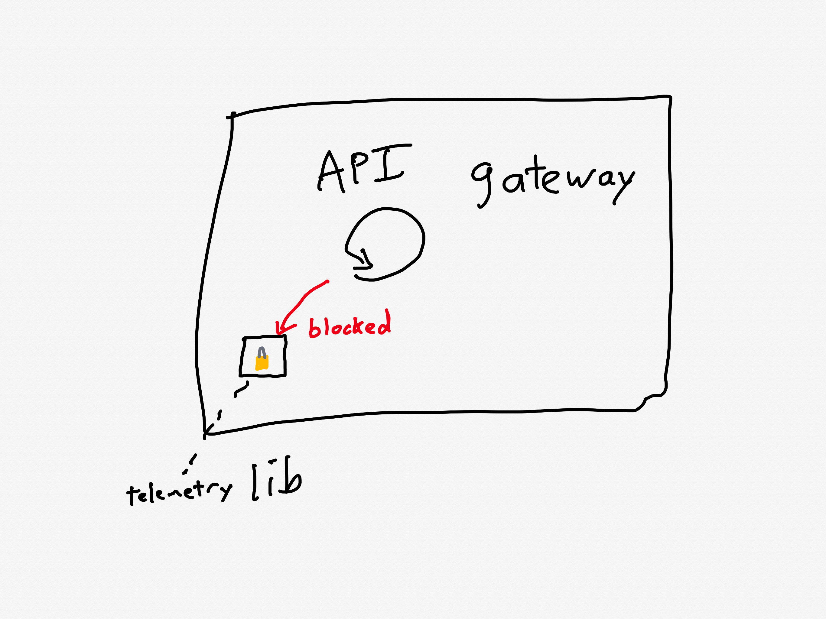

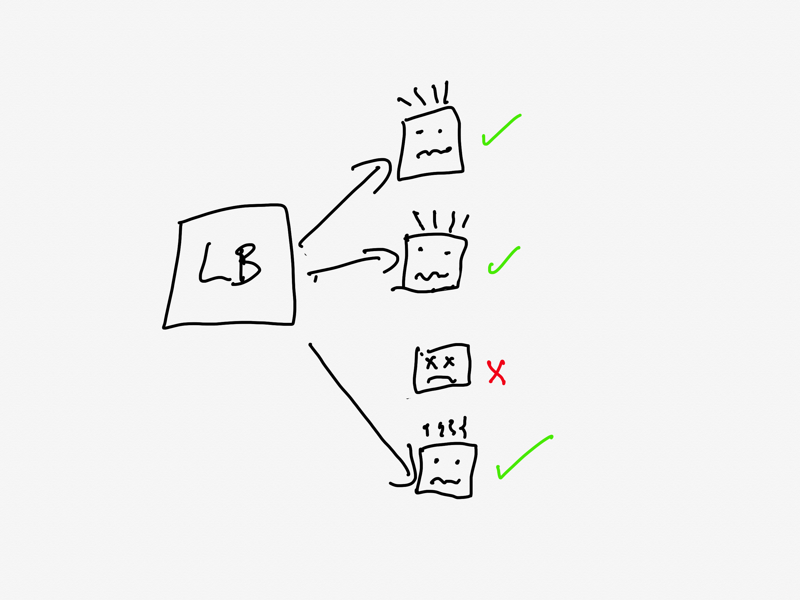


 , and I want a distribution where the probability of a negative TTR is zero. I could just truncate the Gaussian, but instead I decided to go with the Poisson distribution instead, because it doesn’t go negative. Note that the Poisson distribution is discrete where the Gaussian is continuous. The Poisson also has the nice property that it is characterized by only a single parameter (which is called μ in
 ![E[Z] = \frac{\zeta(a-1)}{\zeta(a)}](https://s0.wp.com/latex.php?latex=E%5BZ%5D+%3D+%5Cfrac%7B%5Czeta%28a-1%29%7D%7B%5Czeta%28a%29%7D&bg=ffffff&fg=000000&s=3&c=20201002)


 , which is fantastically small. For the zeta distribution, an incident of 100 minutes is on the order of
  , which is 42 orders of magnitude more likely than the Poisson!


 times more observations than you would compared to if you were sampling from a Gaussian distribution.


