On variability

I was listening to Todd Conklin’s Pre-Accident Investigation Podcast the other day, to the episode titled When Normal Variability Breaks: The ReDonda Story. The name ReDonda in the title refers to ReDonda Vaught, an American registered nurse. In 2017, she was working at the Vanderbilt University Medical Center in Nashville when she unintentionally administered the wrong drug to a patient under her care, a patient who later died. Vaught was fired, then convicted by the state of Tennessee for criminally negligent homicide and abuse of an impaired adult. It’s a terrifying story, really a modern tale of witch-burning, but it’s not what this post is about. Instead, I want to home in a term from the podcast title: normal variability.

In the context of the field of safety, the term variability refers to how human performance is, well, variable. We don’t always do the work the exact same way. This variation happens between humans, where different people will do work in different ways. And the variation also happens within humans, the same person will perform a task differently over time. The sources of variation in human performance are themselves varied: level of experience, external pressures being faced by the person, number of hours of sleep the night before, and so on.

In the old view of safety, there is an explicitly safe way to perform the work, as specified in documented procedures. Follow the procedures, and incidents won’t happen. In the software world, these procedures might be: write unit tests for new code, have the change reviewed by a peer, run end-to-end tests in staging, and so on. Under this view of the world, variability is necessarily a bad thing. Since variability means people do work differently, and since safety requires doing work the proscribed way, human variability is a source of incidents. Traditional automation doesn’t have this variability problem: it always does the work the same way. Hence you get the old joke:

The factory of the future will have only two employees: a man and a dog. The man will be there to feed the dog. The dog will be there to keep the man from touching the equipment.

In the new view of safety, normal variability is viewed as an asset rather than a liability. In this view, the documented procedures for doing the work are always inadequate, they can never capture all of the messy details of real work. It is the human ability to adapt, to change the way that they do the work based on circumstances, that creates safety. That’s why you’ll hear resilience engineering folks use the (positive) term adaptive capacity rather than the (more neutral) human variability, to emphasize that human variability is, quite literally, adaptive. This is why tech companies still staff on-call rotations even though they have complex automation that is supposed to keep things up and running. It’s because the automation can never handle all of the cases that the universe will throw at it. Even sophisticated automation always eventually proves too rigid to be able to handle some particular circumstance that was never foreseen by the designers. This is the perfect-storm, weird-edge-case stuff that post-incident write-ups are made of.

This, again, brings us back to AI.

My own field of software development is being roiled by the adoption of AI-based coding tools like Anthropic’s Claude Code, OpenAI’s Codex, and Google’s Gemini Code Assist. These AI tools are rapidly changing the way that software is being developed, and you can read many blog posts of early adopters who are describing their experiences using these new tools. Just this week, there was a big drop in the market value of multiple software companies; I’ve already seen references to the beginning of the SaaS-Pocalypse, the idea being that companies will write bespoke tools using AI rather than purchasing software from vendors. The field of software development has seen a lot of change in terms of tooling in my own career, but one thing that is genuinely different about these AI-based tools is that they are inherently non-deterministic. You interact with these tools by prompting them, but the same prompt yields different results.

Non-determinism in software development tools is seen as a bad thing. The classic example of non-determinism-as-bad is flaky tests. A flaky test is non-deterministic: the same input may lead to a pass or a fail. Nobody wants non-determinism like this in our test suite. On the build side of things, we hope that our compiler emits the same instructions given the same source file and arguments. There’s even a whole movement around reproducible builds, the goal of which is to stamp out all of the non-determinism in the process of producing binaries from the original source code, where the ideal is achieving bit-for-bit identical binaries. Unsurprisingly, then, the non-determinism of the current breed of AI coding tools is seen as a problem. Here’s a quote from a recent article in the Wall Street Journal by Chip Cutter and Sebastian Herrera: Here’s Where AI Is Tearing Through Corporate America:

Satheesh Ravala is chief technology officer of Candescent, which makes digital technology used by banks and credit unions. He has fielded questions from employees about what innovations like Anthropic’s new features mean for the company, and responded by telling them banks rely on the company for software that does exactly what it’s supposed to every time—something AI struggles with.

“If I want to transfer $10,” he said, “it better be $10 not $9.99.”

I believe the AI coding tools are only going to improve with time, though I don’t feel confident in predicting whether future improvements will be orders-of-magnitude or merely incremental. What I do feel confident in predicting is that the non-determinism in these tools isn’t going away.

At their heart, these tools are sophisticated statistical models: they are prediction machines. When you’re chatting with one, it is predicting the next word to say, and then it feeds back the entire conversation so far, predicts the next word to say again, and so on. Because they are statistical models, there is some probability distribution of next word to predict. You could build the system to always choose the most likely word to say next. Statistical models aren’t just an AI thing, and many statistical models do use such a maximum likelihood approach. But that’s not what LLMs do in general. Instead, there’s some randomness that is intentionally injected into the system so that it doesn’t always just pick the most likely next word, but instead does a biased random selection of the next word, based on the statistical model of what’s most likely to come next, and based on a parameter called temperature, drawing an analogy to physics. If the temperature is zero, then the system always outputs the most likely next word. The higher the temperature, the more random the selection is.

What’s fascinating to me about this is the deliberate injection of randomness improved the output of the models, as judged qualitatively by humans. In other words, increasing the variability of the system improved outcomes.

Now, these LLMs haven’t achieved the level of adaptability that humans possess, though they can certainly perform some impressive cognitive tasks. I wouldn’t say they have adaptive capacity, and I firmly believe that humans will still need to be on-call for software system for the remainder of my career, despite the proliferation of AI SRE solutions. But what I am saying instead is that the ability of LLMs to perform cognitive tasks well depends upon them being able to leverage variability. And my prediction is that this dependence on variability isn’t going to go away. LLMs will get better, and they might even get much better, but I don’t think they’ll ever be deterministic. I think variability is an essential ingredient for a system to be able to perform these sorts of complex cognitive tasks.

Ashby taught us we have to fight fire with fire

There’s an old saying in software engineering, originally attributed to David Wheeler: We can solve any problem by introducing an extra level of indirection. The problem is that indirection adds complexity to a system. Just ask anybody who is learning C and is wrestling with the concept of pointers. Or ask someone who is operating an unfamiliar codebase and is trying to use grep to find the code that relates to certain log messages. Indirection is a powerful tool, but it also renders systems more difficult to reason about.

The old saying points at a more general phenomenon: our engineering solutions to problems invariably add complexity.

Spinning is hard

There was a fun example of this phenomenon that made it to Hacker News the other day. It was a post written by Clément Grégoire of siliceum titled Spinning around: Please don’t!. The post was about the challenges of implementing spin locks.

A spin lock is a type of lock where the thread spins in a loop waiting for the lock to be released so it can grab it. The appeal of a spin-lock is that it should be faster than a traditional mutex lock provided by the operating system: using a spin-lock saves you the performance cost of doing a context switch into the kernel. Grégoire’s initial C++ spin-lock implementation looks basically like this (I made some very minor style changes):

			
class SpinLock {
  int is_locked = 0;
  public:
    void lock() {
      while (is_locked != 0) { /* spin */ }
      is_locked = 1;
    }
    void unlock() { is_locked = 0; }
}

		

As far as locking implementations go, this is a simple one. Unfortunately, it has all sorts of problems. Grégoire’s post goes on to describe these problems, as well as potential solutions, and additional problems created by those proposed solutions. Along the way, he mentions issues such as:

torn reads
race condition
high CPU utilization when not using the dedicated PAUSE (x86) or YIELD (arm) (spin loop hint) instruction
waiting for too long when using the dedicated instruction
contention across multiple cores attempting atomic writes
high cache coherency traffic across multiple core caches
excessive use of memory barriers
priority inversion
false sharing

Below is an implementation that Grégoire proposes to address these issues, with very slight modifications. Note that it requires a system call, so it’s operating-system-specific. He used Windows systems calls, so that’s why I used as well: on Linux, Grégoire notes that you can use the futex API.

(Note: I did not even try to run this code, it’s just to illustrate what the solution looks like)

			
#include <atomic> // for std::atomic
#include <Windows.h> // for WaitOnAddress, WakeByAddressSingle
class SpinLock {
  std::atomic<int32_t> is_locked{0};
  public:
    void lock();
    void unlock(); 
};
void cpu_pause() {
#if defined(__i386__) || defined(__x86_64__) || defined(_M_IX86) || defined(_M_X64)
    _mm_pause();
#elif defined(__arm__) || defined(__aarch64__) || defined(_M_ARM) || defined(_M_ARM64) || defined(_M_ARM64EC)
    __builtin_arm_yield();
#else
    #error "unknown instruction set"
#endif
}
static inline uint64_t get_tsc() {
#if defined(__i386__) || defined(__x86_64__) || defined(_M_IX86) || defined(_M_X64)
    return __rdtsc();
#elif defined(__arm__) || defined(__aarch64__) || defined(_M_ARM) || defined(_M_ARM64) || defined(_M_ARM64EC)
    return __builtin_arm_rsr64("cntvct_el0");
#else
    #error "unknown instruction set"
#endif
}
static inline bool before(uint64_t a, uint64_t b) {
    return ((int64_t)b - (int64_t)a) > 0;
}
struct Yielder {
  static const int maxPauses = 64; // MAX_BACKOFF
  int nbPauses = 1;
  const int maxCycles =/*Some value*/;
  void do_yield_expo_and_jitter() {
    uint64_t beginTSC = get_tsc();
    uint64_t endTSC = beginTSC + maxCycles; // Max duration of the yield
    // jitter is in the range of [0;nbPauses-1].
    // We can use bitwise AND since nbPauses is a power of 2.
    const int jitter = static_cast<int>(beginTSC & (nbPauses - 1));
    // So subtracting we get a value between [1;nbPauses]
    const int nbPausesThisLoop = nbPauses - jitter;
    for (int i = 0; i < nbPausesThisLoop && before(get_tsc(), endTSC); i++)
      cpu_pause();
    // Multiply the number of pauses by 2 until we reach the max backoff count.
    nbPauses = nbPauses < maxPauses ? nbPauses * 2 : nbPauses;
  }
   void do_yield(int32_t* address, int32_t comparisonValue, uint32_t timeoutMs) {
    do_yield_expo_and_jitter();
    if (nbPauses >= maxPauses) {
      WaitOnAddress(address, &comparisonValue, sizeof(comparisonValue), timeoutMs);
      nbPauses = 1;
    }
  }
};
void SpinLock::lock() {
    Yielder yield;
    // Actually start by an exchange, we assume the lock is not already taken
    // This is because the main use case of a spinlock is when there's no contention!
    while (is_locked.exchange(1, std::memory_order_acquire) != 0)
    {
        // To avoid locking the cache line with a write access, always only read before attempting the writes
        do {
            yield.do_yield(&is_locked, 1 /*while locked*/ , 1 /*ms*/);
        } while (is_locked.load(std::memory_order_relaxed) != 0);
    }
}
void SpinLock::unlock() {
  is_locked = 0;
  WakeByAddressSingle(&is_locked); // Notify a potential thread waiting, if any  
}

		

Yeesh, this is a lot more complex than our original solution! And yet, that complexity exists to address real problems. It uses dedicated hardware instructions for spin-looping more efficiently, it uses exponential backoff with jittering to reduce contention across cores, it takes into account memory ordering to eliminate unwanted barriers, and it uses special system calls to help the system calls schedule the threads more effectively. The simplicity of this initial solution was no match for the complexity of modern multi-core NUMA machines. No matter how simple that initial solution looked as a C++ program, the solution must interact with the complexity of the fundamental building blocks of compilers, operating systems, and hardware architecture.

Flying is even harder

Now let’s take an example from outside of software: aviation. Consider the following two airplanes: a WWI era Sopwith Camel, and a Boeing 787 Dreamliner.

While we debate endlessly over what we mean by complexity, I feel confident in claiming that the Dreamliner is a more complex airplane than the Camel. Heck, just look at the difference in the engines used by the two planes: the Clerget 9B for the Camel, and the GE GEnx for the Dreamliner.

Image attributions
Sopwith Camel: Airwolfhound, CC BY-SA 2.0 via Wikimedia Commons
Boeing 787 Dreamliner: pjs2005 from Hampshire, UK, CC BY-SA 2.0 via Wikimedia Commons
Clerget 9B: Nimbus227, Public domain, via Wikimedia Commons
GE Genx: Olivier Cleynen, CC BY-SA 3.0 via Wikimedia Commons

And, yet, despite the Camel being simpler than the Dreamliner, the Camel was such a dangerous airplane to fly that almost as many Camel pilots died flying it in training as were killed flying in combat! The Dreamliner is both more complex and safer. The additional complexity is doing real work here, it contributes to making the Dreamliner safer.

Complexity: threat or menace?

But we’re also right to fear complexity. Complexity makes it harder for us humans to reason about the behavior of systems. Evolution has certainly accomplished remarkable things in designing biological systems: these systems are amazingly resilient. One thing they aren’t, though, is easy to understand, as any biology major will tell you.

Complexity also creates novel failure modes. The Dreamliner itself experienced safety issues related to electrical fires: a problem that Camel pilots never had to worry about. And there were outright crashes where software complexity was a contributing factor, such as Lion Air Flight 610, Ethiopian Airlines Flight 302 (both Boeing 737 MAX aircraft), and Air France Flight 447 (an Airbus A330).

Unfortunately for us, making systems more robust means adding complexity. An alternate formulation of the saying at the top of this post is: All problems in computer science can be solved by another level of indirection, except for the problem of too many layers of indirection. Complexity solves all problems except the problem of complexity.

The psychiatrist and cybernetician W. Ross Ashby expressed this phenomenon as a law, which he called the Law of Requisite Variety. Today it’s also known as Ashby’s Law. Ashby noted that when you’re building a control system, the more complex the problem space is, the more complex your controller needs to be. For example, a self-driving car is necessarily going to have a much more complex control system than a thermostat.

When faced with a complex problem, we have to throw complexity at it in order to solve it.

This blog is called surfing complexity because I want to capture the notion that we will always have to deal with complexity: we can’t defeat it, but we can get better at navigating through it effectively.

And that brings us, of course, to AI.

Throwing complexity back at the computer

Modern LLM systems are enormously complex. OpenAI, Anthropic, and Google don’t publish parameter counts for their models anymore, but Meta’s Llama 4 has 17 billion active parameters, and either 109 or 400 billion total parameters, depending on the model. These systems are so complex that trying to understand their behavior looks more like biology research than engineering.

One type of task that LLMs are very good at solving are the kind of problem that exist solely because of computers in. For example, have you ever struggled to align content the right way in a Word document? It’s an absolute exercise in frustration. My wife threw this problem at an LLM and it fixed up the formatting for her. I’ve used LLMs for various tasks myself, including asking it do development tasks, and using it like a search engine to answer questions. And sometimes it works well, and sometimes it doesn’t. But where’ve find that these tools really shine is when I’ve got some batch of data, maybe a log file or a CSV or some JSON, and I want it do some processing task, like change the shape of it, or extract some data, so I can feed it into some other thing. I don’t ask it for the output directly, instead I ask it to generate a shell script or a Perl one-liner that’ll do the ad-hoc task, and then I run it. And, like the Word problem, I have a problem that was created by a computer that I need to solve.

I’m using this enormously complex system, an LLM, to help me solve a problem that was created by software complexity in the first place.

Back in March 2016, Tom Limoncelli wrote a piece for ACM Queue titled Automation Should Be Like Iron Man, Not Ultron. Drawing inspiration from John Allspaw in particular, and Cognitive Systems Engineering in general, Limoncelli argued that automation should be written to be directable by humans rather than acting fully independently. He drew an analogy to Iron Man’s suit being an example of good automation, and the robot villain Ultron being an example of bad automation. Iron Man’s suit enables him to do things he couldn’t do otherwise, but he remains in control of it, and he can direct it to do the things he needs it to do. Ultron is an autonomous agent that was built for defensive purposes but ends up behaving unexpectedly, causing more problems than it solves. But my recent experiences with LLMs have led me to a different analogy: Tron.

In the original movie, Tron is a good computer program that fights the bad computer programs. In particular, he’s opposed to the Master Control Program, an evil AI who is referred to as the MCP. (Incidentally, this is what a Gen Xer like me automatically thinks of when hearing the term “MCP”). Tron struggles against the MCP on behalf of the humans, who create and use the programs. He fights for the users.

I frequently describe my day-to-day work as “fighting with the computer”. On some days I win the fight, and on some days I lose. AI tools have not removed the need to fight with the computer to get my work done. But now I can send an AI agent to fight some of these battles for me. There’s a software agent who will fight with other software on my behalf. They haven’t reduced the overall complexity of the system. In fact, if you take into account the LLM’s complexity, the overall system complexity is much larger. But I’m deploying this complexity in an Ashby-ian sense, to help defeat other software complexity so I can get my work done. Like Tron, it fights for the user.

Amdahl, Gustafson, coding agents, and you

In the software operations world, if your service is successful, then eventually the load on it is going to increase to the point where you’ll need to give that services more resources. There are two strategies for increasing resources: scale up and scale out.

Scaling up means running the service on a beefier system. This works well, but you can only scale up so much before you run into limits of how large a machine you have access to. AWS has many different instance types, but there will come a time when even the largest instance type isn’t big enough for your needs.

The alternative is scaling out: instead of running your service on a bigger machine, you run your service on more machines, distributing the load across those machines. Scaling out is very effective if you are operating a stateless, shared-nothing microservice: any machine can service any request. It doesn’t work as well for services where the different machines need to access shared state, like a distributed database. A database is harder to scale out because the machines need to share state, which means they need to coordinate with each other.

Once you have to do coordination, you no longer get a linear improvement in capacity based on the number of machines: doubling the number of machines doesn’t mean you can handle double the load. This comes up in scientific computing applications, where you want to run a large computing simulation, like a climate model, on a large-scale parallel computer. You can run independent simulations very easily in parallel, but if you want to run an individual simulation more quickly, you need to break up the problem in order to distribute the work across different processors. Imagine modeling the atmosphere as a huge grid, and dividing up that grid and having different processors work on simulating different parts of the grid. You need to exchange information between processors at the grid boundaries, which introduces the need for coordination. Incidentally, this is why supercomputers have custom networking architectures, in order to try to reduce these expensive coordination costs.

In the 1960s, the American computer architect Gene Amdahl made the observation that the theoretical performance improvement you can get from a parallel computer is limited by the fraction of work that cannot be parallelized. Imagine you have a workload where 99% of the work is amenable to parallelization, but 1% of it can’t be parallelized:

Let’s say that running this workload on a single machine takes 100 hours. Now, if you ran this on an infinitely large supercomputer, the green part above would go from 99 hours to 0. But you are still left with the 1 hour of work that you can’t parallelize, which means that you are limited to 100X speedup no matter how large your supercomputer is. The upper limit on speedup based on the amount of the workload that is parallelizable is known today as Amdahl’s Law.

But there’s another law about scalability on parallel computers, and it’s called Gustafson’s Law, named for the American computer scientist John Gustafson. Gustafson observed that people don’t just use supercomputers to solve existing problems more quickly. Instead, they exploit the additional resources available in supercomputers to solve larger problems. The larger the problem, the more amenable it is to parallelization. And so Gustafson proposed scaled speedup as an alternative metric, which takes this into account. As he put it: in practice, the problem size scales with the number of processors.

And that brings us to LLM-based coding agents.

AI coding agents improve programmer productivity: they can generate working code a lot more quickly than humans can. As a consequence of this productivity increase, I think we are going to find the same result that Gustafson observed at Sandia National Labs: that people will use this productivity increase in order to do more work, rather than simply do the same amount of coding work with fewer resources. This is a direct consequence of the law of stretched systems from cognitive systems engineering: systems always get driven to their maximum capacity. If coding agents save you time, you’re going to be expected to do additional work with that newfound time. You launch that agent, and then you go off on your own to do other work, and then you context-switch back when the agent is ready for more input.

And that brings us back to Amdahl: coordination still places a hard limit on how much you can actually do. Another finding from cognitive systems engineering is that coordination costs, continually. Coordination work require requires continuous investment of effort. The path we’re on feels the work of software development is shifting from direct coding to a human coordinating with a single agent to a human coordinating work among multiple agents working in parallel. It’s possible that we will be able to fully automate this coordination work, by using agents to do the coordination. Steve Yegge’s Gas Town project is an experiment to see how far this sort of automated agent-based coordination can go. But I’m pessimistic on this front. I think that we’ll need human software engineers to coordinate coding agents for the foreseeable future. And the law of stretched systems teaches us that these multi-coding-agent systems are going to keep scaling up the number of agents until the human coordination work becomes the fundamental bottleneck.

From Rasmussen to Moylan

I hadn’t heard of James Moylan until I read a story about him in the Wall Street Journal after he passed away in December, but it turns out my gaze had fallen on one his designs almost every day of my adult life. Moylan was the designer at Ford who came up with the idea of putting an arrow next to the gas tank symbol to indicate which side of the car the tank was on. It’s called the Moylan Arrow in his honor.

The Moylan Arrow put me in mind of another person we lost in 2025, the safety researcher James Reason. If you’ve heard of James Reason, it’s probably because of the Swiss cheese model of accidents that Reason proposed. But Reason made other conceptual contributions to the field of safety, such as organizational accidents and resident pathogens. The contribution that inspired this post was his model of human error described in his book Human Error. The model is technically called the Generic Error-Modeling System (GEMS), but I don’t know if anybody actually refers to it by that name. And the reason GEMS came to mind was because Reason’s model was itself built on top of another researcher’s model of human performance, Jens Rasmussen’s Skills, Rules and Knowledge (SRK) model.

Rasmussen was trying to model how skilled operators perform tasks, how they process information in order to do so, and how user interfaces like control panels could better support their work. He worked at a Danish research lab focused on atomic energy, and his previous work included designing a control room for a Danish nuclear reactor, as well as studying how technicians debugged problems in electronics circuits.

The part of the SRK model that I want to talk about here is the information processing aspect. Rasmussen draws a distinction between three different types of information, which he labels signals, signs, and symbols.

The signal is the most obvious type of visual information to absorb, where there is minimal interpretation required to make sense of the signal. Consider the example of the height of mercury in a thermometer to observe the temperature. There’s a direct mapping between the visual representation of the sensor and the underlying phenomenon in the environment – a higher level of mercury means a hotter temperature.

A sign requires some background knowledge in order to interpret the visual information, but once you have internalized that information, you will be able to very quickly to interpret its meaning sign. Traffic lights are one such example: there’s no direct physical relationship between a red-colored light and the notion of “stop”, it’s an indirect association, mediated by cultural knowledge.

A symbol requires more active cognitive work in order to make sense of. To take an example from my own domain, reading the error logs emitted by a service would be an example of a task that involves visual information processing of symbols. Interpreting log error messages are much more laborious than, say, interpreting a spike in an error rate graph.

(Note: I can’t remember exactly where I got the thermometer and traffic light examples from, but I suspect it was from A Meaning Processing Approach to Cognition by John Flach and Fred Voorhost).

From his paper, Rasmussen describes signals as representing continuous variables. That being said, I propose the Moylan arrow as a great example of a signal, even though the arrow does not represent a continuous variable. Moylan’s arrow doesn’t require background knowledge to learn how to interpret it, because there’s a direct mapping between the direction the triangle is pointing and the location of the gas tank.

Rasmussen maps these three types of information processing to three types of behavior (signals relate to skill-based behavior, signs relate to rule-based behavior, and symbols relate to knowledge-based behavior). James Reason created an error taxonomy based on these different behaviors. In Reason’s terminology, slips and lapses happen at the skill-based level, rule-based mistakes happen at the rule-based level, and knowledge-based mistakes happen at the knowledge-based level.

Rasmussen’s original SRK paper is a classic of the field. Even though it’s forty years old, because the focus is on human performance and information processing, I think it’s even more relevant today than when it was originally published: thanks to open source tools like Grafana and the various observability vendors out there, there are orders of magnitude more operator dashboards being designed today than there were back in the 1980s. While we’ve gotten much better at being able to create dashboards, I don’t think my field has advanced much at being able to create effective dashboards.

Brief thoughts on the recent Cloudflare outage

I was at QCon SF during the recent Cloudflare outage (I was hosting the Stories Behind the Incidents track), so I hadn’t had a real chance to sit down and do a proper read-through of their public writeup and capture my thoughts until now. As always, I recommend you read through the writeup first before you read my take.

All quotes are from the writeup unless indicated otherwise.

Hello saturation my old friend

The software had a limit on the size of the feature file that was below its doubled size. That caused the software to fail.

One thing I hope readers take away from this blog post is the complex systems failure mode pattern that resilience engineering researchers call saturation. Every complex system out there has limits, no matter how robust that system is. And the systems we deal with have many, many different kinds of limits, some of which you might only learn about once you’ve breached that limit. How well a system is able to perform as it approaches one of its limits is what resilience engineering is all about.

Each module running on our proxy service has a number of limits in place to avoid unbounded memory consumption and to preallocate memory as a performance optimization. In this specific instance, the Bot Management system has a limit on the number of machine learning features that can be used at runtime. Currently that limit is set to 200, well above our current use of ~60 features.

In this particular case, the limit was set explicitly.

thread fl2_worker_thread panicked: called Result::unwrap() on an Err value

As sparse as the panic message is, it does explicitly tell you that the problematic call site was an unwrap call. And this is one of the reasons I’m a fan of explicit limits over implicit limits: you tend to get better error messages than when breaching an implicit limit (e.g., of your language runtime, the operating system, the hardware).

A subsystem designed to protect surprisingly inflicts harm

Identify and mitigate automated traffic to protect your domain from bad bots. – Cloudflare Docs

The problematic behavior was in the Cloudflare Bot Management system. Specifically, it was in the bot scoring functionality, which estimates the likelihood that a request came from a bot rather than a human.

This is a system that is designed to help protect their customer from malicious bots, and yet it ended up hurting their customers in this case rather than helping them.

As I’ve mentioned previously, once your system achieves a certain level of reliability, it’s the protective subsystems that end up being things that bite you! These subsystems are a net positive, they help much more than they hurt. But they also add complexity, and complexity introduces new, confusing failure modes into the system.

The Cloudflare case is a more interesting one than the typical instances of this behavior I’ve seen, because Cloudflare’s whole business model is to offer different kinds of protection, as products for their customers. It’s protection-as-a-service, not an internal system for self-protection. But even though their customers are purchasing this from a vendor rather than building it in-house, it’s still an auxiliary system intended to improve reliability and security.

Confusion in the moment

What impressed me the most about this writeup is that they documented some aspects of what it was like responding to this incident: what they were seeing, and how they tried to made sense of it.

In the internal incident chat room, we were concerned that this might be the continuation of the recent spate of high volume Aisuru DDoS attacks:

Man, if I had a nickel every time I saw someone Slack “Is it DDOS?” in response to a surprising surge of errors returned by the system, I could probably retire at this point.

The spike, and subsequent fluctuations, show our system failing due to loading the incorrect feature file. What’s notable is that our system would then recover for a period. This was very unusual behavior for an internal error.

We humans are excellent at recognizing patterns based on our experience, and that generally serves us well during incidents. Someone who is really good at operations can frequently diagnose the problem very quickly just by, say, the shape of a particular graph on a dashboard, or by seeing a specific symptom and recalling similar failures that happened recently.

However, sometimes we encounter a failure mode that we haven’t seen before, which means that we don’t recognize the signals. Or we might have seen a cluster of problems recently that followed a certain pattern, and assume that the latest one looks like the last one. And these are the hard ones.

This fluctuation made it unclear what was happening as the entire system would recover and then fail again as sometimes good, sometimes bad configuration files were distributed to our network. Initially, this led us to believe this might be caused by an attack.

This incident was one of those hard ones: the symptoms were confusing. The “problem went away, then came back, then went away again, then came back again” type of unstable incident behavior is generally much harder to diagnose than one where the symptoms are stable.

Throwing us off and making us believe this might have been an attack was another apparent symptom we observed: Cloudflare’s status page went down. The status page is hosted completely off Cloudflare’s infrastructure with no dependencies on Cloudflare. While it turned out to be a coincidence, it led some of the team diagnosing the issue to believe that an attacker may be targeting both our systems as well as our status page.

Here they got bit by a co-incident, an unrelated failure of their status page that led them to believe (reasonably!) that the problem must have been external.

I’m still curious as to what happened with their status page. The error message they were getting mentions CloudFront, so I assume they were hosting their status page on AWS. But their writeup doesn’t go into any additional detail on what the status page failure mode was.

But the general takeaway here is that even the most experienced operators are going to take longer to deal with a complex, novel failure mode, precisely because it is complex and novel! As the resilience engineering folks say, prepare to be surprised! (Because I promise, it’s going to happen).

A plea: assume local rationality

The writeup included a screenshot of the code that had an unhandled error. Unfortunately, there’s nothing in the writeup that tells us what the programmer was thinking when they wrote that code.

In the absence of any additional information, a natural human reaction is to just assume that the programmer was sloppy. But if you want to actually understand how these sorts of incidents actually happen, you have to fight this reaction.

People always make decisions that make sense to them in the moment, based on what they know and what constraints they are operating under. After all, if that wasn’t true, then they wouldn’t have made that decision. The only we can actually understand the conditions that enable incidents, we need to try as hard as we can to put ourselves into the shoes of the person who made that call, to understand what their frame of mind was at the moment.

If we don’t do that, we risk the problem of distancing through differencing. We say, “oh, those devs were bozos, I would never have made that kind of mistake”. This is a great way to limit how much you can learn from an incident.

Detailed public writeups as evidence of good engineering

The writeup produced by Cloudflare (signed by the CEO, no less!) was impressively detailed. It even includes a screenshot of a snippet of code that contributed to the incident! I can’t recall ever reading another public writeup with that level of detail.

Companies generally err on the side of saying less rather than more. After all, if you provide more detail, you open yourself up to criticism that the failure was due to poor engineering. The fewer details you provide, the fewer things people can call you out on. It’s not hard to find people online criticizing Cloudflare online using the details they provided as the basis for their criticism.

Now, I think it would advance our industry if people held the opposite view: the more details that are provided an incident writeup, the higher esteem we should hold that organization. I respect Cloudflare is an engineering organization a lot more precisely because they are willing to provide these sorts of details. I don’t want to hear what Cloudflare should have done from people who weren’t there, I want to hear us hold other companies up to Cloudflare’s standard for describing the details of a failure mode and the inherently confusing nature of incident response.

My favorite developer productivity research method that nobody uses

You’ve undoubtedly heard of the psychological concept called flow state. This is the feeling you get when you’re in the zone, where you’re doing some sort of task, and you’re just really into it, and you’re focused, and it’s challenging but not frustratingly so. It’s a great feeling. You might experience this with a work task, or a recreational one, like when playing a sport or a video game. The pioneering researcher on the phenomenon of flow was the Hungarian-American psychologist Mihaly Csikszentmihalyi, and he wrote a popular book on the subject back in 1990 with the title Flow: The Psychology of Optimal Experience, which I read many years ago. But the one thing that stuck around most with me from Csikszentmihalyi’s book on Flow was the research method that he used to study flow.

One of the challenges of studying people’s experiences is that it’s difficult for researchers to observe them directly. This problem comes up when an organization tries to do research on the current state of developer productivity within the organizations. I harp on “make work visible” a lot because so much of the work we do in the software world is so hard for others to see. There are different data collection techniques that developer productivity researchers use, including surveys, interviews, focus groups, as well as automatic collection of metrics, like the DORA metrics. Of those, only the automatic collection of metrics focuses on in-the-moment data, and it’s a very thin type of data at that. Those metrics can’t give you any insights into the challenges that your developers are facing.

My preferred technique is the case study, which I try to apply to incidents. I like the incident case study technique because it gives us an opportunity to go deep into the nature of the work for a specific episode. But incident-as-case-study only works for, well, incidents, and while a well-done incident case study can shine a light on the nature of the development work, there’s also a lot that it will miss.

Csikszentmihalyi used a very clever approach which was developed by his PhD student Suzanne Prescott, called experience sampling. He gave the participants of his study pagers, and he would page them at random times. When paged, the participants would write down information about their experiences in a journal in-the-moment. In this way, he was able to collect information about subjective experience, without the problems you get when trying to elicit an account retrospectively.

I’ve never read about anybody trying to use this approach to study developer productivity, and I think that’s a shame. It’s something I’ve wanted to try myself, except that I have not worked in the developer productivity space for a long, long time.

These days, I’d probably use slack rather than a pager and journal to randomly reach out to the volunteers during the study and collect their responses, but the principle is the same. I’ve long wanted to capture an “are you currently banging your head against a wall” metric from developers, but with experience sampling, you could capture a “what are you currently banging your head against the wall about?”

Would this research technique actually work for studying developer productivity issues within an organization? I honestly don’t know. But I’d love to see someone try.

Note: I originally had the incorrect publication date for the Flow book. Thanks to Daniel Miller for the correction.

Easy will always trump simple

One of the early criticisms of Darwin’s theory of evolution by natural selection was about how it could account for the development of complex biological structures. It’s often not obvious to us how the earlier forms of some biological organ would have increase fitness. “What use”, asked the 19th century English biologist St. George Jackson Mivart, “is half a wing?”

One possible answer is that while half a wing might not be useful for flying, it may have had a different function, and evolution eventually repurposed that half-wing for flight. This concept, that evolution can take some existing trait in an organism that serves a function and repurpose it to serve a different function, is called exaptation.

Biology seems to be quite good at using the resources that it has at hand in order to solve problems. Not too long ago, I wrote a review of the book How Life Works: A User’s Guide to the New Biology by the British science writer Philip Ball. One of the main themes of the book is how biologists’ view of genes has shifted over time from the idea DNA-as-blueprint to DNA-as-toolbox. Biological organisms are able to deal effectively with a wide range of challenges by having access to a broad set of tools, which they can deploy as needed based on their circumstances.

We’ll come back to the biology, but for a moment, let’s talk about software design. Back in 2011, Rich Hickey gave a talk at the (sadly defunct) Strange Loop conference with the title Simple Made Easy (transcript, video). In this talk, Hickey drew a distinction between the concepts of simple and easy. Simple is the opposite of complex, where easy is something that’s familiar to us: the term he used to describe the concept of easy that I really liked was at hand. Hickey argues that when we do things that are easy, we can initially move quickly, because we are doing things that we know how to do. However, because easy doesn’t necessarily imply simple, we can end up with unnecessarily complex solutions, which will slow us down in the long run. Hickey instead advocates for building simple systems. According to Hickey, simple and easy aren’t inherently in conflict, but are instead orthogonal. Simple is an absolute concept, and easy is relative to what the software designer already knows.

I enjoy all of Rich Hickey’s talks, and this one is no exception. He’s a fantastic speaker, and I encourage you to listen to it (there are some fun digs at agile and TDD in this one). And I agree with the theme of his talk. But I also think that, no matter how many people listen to this talk and agree with it, easy will always win out over simple. One reason is the ever-present monster that we call production pressure: we’re always under pressure to deliver our work within a certain timeframe, and easier solutions are, by definition, going to be ones that are faster to implement. That means the incentives on software developers tilts the scales heavily towards the easy side. Even more generally, though, easy is just too effective a strategy for solving problems. The late MIT mathematics professor Gian-Carlo Rota noted that every mathematician has only a few tricks, and that includes famous mathematicians like Paul Erdős and David Hilbert.

Let’s look at two specific examples of the application of easy from the software world, specifically, database systems. The first example is about knowledge that is at-hand. Richard Hipp implemented the SQLite v1 as a compiler that would translate SQL into byte code, because he had previous experience building compilers but not building database engines. The second example is about an exaptation, leveraging an implementation that was at-hand. Postgres’s support for multi-version concurrency control (MVCC) relies upon an implementation that was originally designed for other features, such as time-travel queries. (Multi-version support was there from the beginning, but MVCC was only added in version 6.5).

Now, the fact that we rely frequently on easy solutions doesn’t necessarily mean that they are good solutions. After all, the Postgres source I originally linked to has the title The Part of PostgreSQL We Hate the Most. Hickey is right that easy solutions may be fast now, but they will ultimately slow us down, as the complexity accretes in our system over time. Heck, one of the first journal papers that I published was a survey paper on this very topic of software getting more difficult to maintain over time. Any software developer that has worked at a company other than a startup has felt the pain of working with a codebase that is weighed down by what Hickey refers to in his talk as incidental complexity. It’s one of the reasons why startups can move faster than more mature organizations.

But, while companies are slowed down by this complexity, it doesn’t stop them entirely. What Hickey refers to in his talk as complected systems, the resilience engineering researcher David Woods refers to as tangled. In the resilience engineering view, Woods’s tangled, layered networks inevitably arise in complex systems.

Hickey points out that humans can only keep a small number of entities in their head at once, which puts a hard limit on our ability to reason about our systems. But the genuinely surprising thing about complex systems, including the ones that humans build, is that individuals don’t have to understand the system for them to work! It turns out that it’s enough for individuals to only understand parts of the system. Even without anyone having a complete understanding of the whole system, we humans can keep the system up and running, and even extend its functionality over time.

Now, there are scenarios when we do need to bring to bear an understanding of the system that is greater than any one person possesses. My own favorite example is when there’s an incident that involves an interaction between components, where no one person understands all of the components involved. But here’s another thing that human beings can do: we can work together to perform cognitive tasks that none of us could do on their own, and one such task is remediating an incident. This is an example of the power of diversity, as different people have different partial understandings of the system, and we need to bring those together.

To circle back to biology: evolution is terrible at designing simple systems: I think biological systems are the most complex systems that we humans have encountered. And yet, they work astonishingly well. Now, I don’t think that we should design software the way that evolution designs organisms. Like Hickey, I’m a fan of striving for simplicity in design. But I believe that complex systems, whether you call them complected or tangled, are inevitable, they’re just baked in to the fabric of the adaptive universe. I also believe that easy is such a powerful heuristic that it is also baked in to how we build and involved systems. That being said, we should be inspired, by both biology and Hickey, to have useful tools at-hand. We’re going to need them.

Cloudflare and the infinite sadness of migrations

(With apologies to The Smashing Pumpkins)

A few weeks ago, Cloudflare experienced a major outage of their popular 1.1.1.1 public DNS resolver.

Technically, the DNS resolver itself was working just fine: it was (as far as I’m aware) up and running the whole time. The problem was that nobody on the Internet could actually reach it. The Cloudflare public write-up is quite detailed, and I’m not going to summarize it here. I do want to bring up one aspect of their incident, because it’s something I worry about a lot from a reliability perspective: migrations.

Cloudflare’s migration

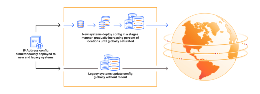
When this incident struck, Cloudflare supported two different ways of managing what they call service topologies. There was a newer system that supported progressive rollout, and an older system where the changes occurred globally. The Cloudflare incident involved the legacy system, which makes global changes, which is why the blast radius of this incident was so large.

Source: https://blog.cloudflare.com/cloudflare-1-1-1-1-incident-on-july-14-2025/

Cloudflare engineers were clearly aware that these sorts of global changes are dangerous. After all, I’m sure that’s one of the reasons why they built their new system in the first place. But migrating all of the way to the new thing takes time.

Migrations and why I worry about them

If you’ve ever worked at any sort of company that isn’t a startup, you’ve had to deal with a migration. Sometimes a migration impacts only a single team that owns the system in question, but often migrations are changes that are large in scope (typically touching many teams) which, while providing new capabilities to the organization as a whole, don’t provide much short-term benefit to the teams who have to make a change to accommodate the migration.

A migration is a kind of change that, almost by definition, the system wasn’t originally designed to accommodate. We build our systems to support making certain types of future changes, and migrations are exactly not these kinds of changes. Each migration is typically a one-off type of change. While you’ll see many migrations if you work at a more mature tech company, each one will be different enough that you won’t be able to leverage common tooling from one migration to help make the next one easier.

All of this adds up to reliability risk. While a migration-related change wasn’t a factor in the Cloudflare incident, I believe that such changes are inherently risky, because you’re making a one-off change to the way that your system works. Developers generally have a sense that these sorts of changes are risky. As a consequence, for an individual on a team who has to do work to support somebody else’s migration, all of the incentives push them towards dragging their feet: making the migration-related change takes time away from their normal work, and increases the risk they break something. On the other hand, completing the migration generally doesn’t provide them short-term benefit. The costs typically outweigh the benefits. And so all of the forces push towards migrations taking a long time.

But a delay in implementing a migration is also a reliability risk, since migrations are often used to improve the reliability of the system. The Cloudflare incident is a perfect example of this: the newer system was safer than the old one, because it supported staged rollout. And while they ran the new system, they had to run the old one as well.

Why run one system when you can run two?

The scariest type of migration to me is the big bang migration, where you cut over all at once from the old system to the new one. Sometimes you have no choice, but it’s an approach that I personally would avoid whenever possible. The alternative is to do incremental migration, migrating parts of the system over time. To do incremental migration, you need to run the old system and the new system concurrently, until you’ve completely finished the migration and can shut the old system down. When I worked at Netflix, people used the term Roman riding to refer to running the old and new system in parallel, in reference to a style of horseback riding.

The problem with Roman riding is that it’s risky as well. While incremental is safer than big bang, running two systems concurrently increases the complexity of the system. There are many, many opportunities for incidents while you’re in the midst of a migration running the two systems in parallel.

What is to be done?

I wish I had a simple answer here. But my unsatisfying one is that engineering organizations at tech companies need to make migrations a part of their core competency, rather than seeing them as one-off chores. I frequently joke that platform engineering should really be called migration engineering, because any org large enough to do platform engineering is going to be spending a lot of its cycles doing migrations.

Migrations are also unglamorous work: nobody’s clamoring for the title of migration engineer. People want to work on greenfield projects, not deal with the toil of a one-off effort to move the legacy thing onto the new thing. There’s also not a ton written on doing migrations. A notable exception is (fellow TLA+ enthusiast) Marianne Bellotti’s book Kill It With Fire, which sits on my bookshelf, and which I really should re-read.

I’ll end this post with some text from the “Remediation and follow-up steps” of the Cloudflare writeup:

We are implementing the following plan as a result of this incident:

Staging Addressing Deployments: Legacy components do not leverage a gradual, staged deployment methodology. Cloudflare will deprecate these systems which enables modern progressive and health mediated deployment processes to provide earlier indication in a staged manner and rollback accordingly.

Deprecating Legacy Systems: We are currently in an intermediate state in which current and legacy components need to be updated concurrently, so we will be migrating addressing systems away from risky deployment methodologies like this one. We will accelerate our deprecation of the legacy systems in order to provide higher standards for documentation and test coverage.

I’m sure they’ll prioritize this particular migration because of the attention garnered on it from this incident. But I also bet there are a whole lot more in-flight migrations at Cloudflare, as well as at other companies, that increase complexity through maintaining two systems and delaying moving to the safer thing. What are they actually going to do in order to complete those other migrations more quickly? If it was easy, it would already be done.

Dijkstra never took a biology course

Simplicity is prerequisite for reliability. — Edsger W. Dijkstra

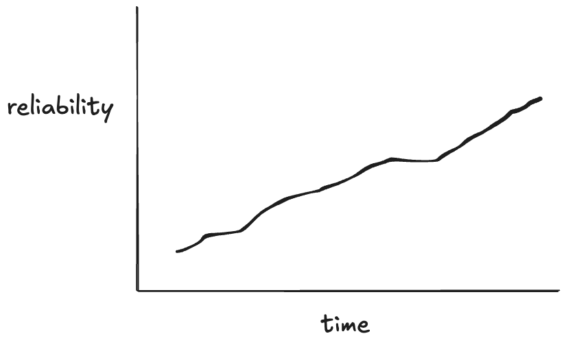
Think about a system whose reliability had significantly improved over some period of time. The first example that comes to my mind is commercial aviation, but I’d encourage you to think of a software system you’re familiar with, either as a user (e.g., Google, AWS) or as a maintainer of a system that’s gotten more reliable over time.

Think of a system where the reliability trend looks like this

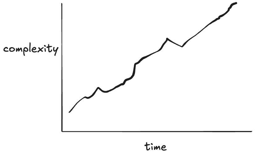
Now, for the system you have thought about where its reliability increased over time, think about what the complexity trend looks like over time for that system. I’d wager you’d see a similar sort of trend.

My claim about what the complexity trend looks like over time

Now, in general, increases in complexity don’t lead to increases in reliability. In some cases, engineers make a deliberate decision to trade off reliability for new capabilities. The telephone system today is much less reliable than it was when I was younger. As someone who grew up in the 80s and 90s, the phone system was so reliable that it was shocking to pick up the phone and not hear a dial tone. We were more likely to experience a power failure than a telephony outage, and the phones still worked when the power was out! I don’t think we even knew the term “dropped call”. Connectivity issues with cell phones are much more common than they ever were with landlines. But this was a deliberate tradeoff: we gave up some reliability in order to have ubiquitous access to a phone.

Other times, the increase in complexity isn’t the product of an explicit tradeoff but rather an entropy-like effect of a system getting more difficult to deal with over time as it accretes changes. This scenario, the one that most people have in mind when they think about increasing complexity in their system, is synonymous with the idea of tech debt. With tech debt the increase in complexity makes the system less reliable, because the risk of making a breaking change in the system has increased. I started this blog post with a quote from Dijkstra about simplicity. Here’s another one, along the same lines, from C.A.R. Hoare’s Turing Award Lecture in 1980:

There are two ways of constructing a software design: One way is to make it so simple that there are obviously no deficiencies, and the other way is to make it so complicated that there are no obvious deficiencies. The first method is far more difficult.

What Dijkstra and Hoare are saying is: the easier a software system is to reason about, the more likely it is to be correct. And this is true: when you’re writing a program, the simpler the program is, the more likely that you are to get it right. However, as we scale up from individual programs to systems, this principle breaks down. Let’s see how that happens.

Djikstra claims simplicity is a prerequisite for reliability. According to Dijkstra, if we encounter a system that’s reliable, it must be a simple system, because simplicity is required to achieve reliability.

reliability ⇒ simplicity

The claim I’m making in this post is the exact opposite: systems that improve in reliability do so by adding features that improves reliability, but come at the cost of increased complexity.

reliability ⇒ complexity

Look at classic works on improving the reliability of real-world systems like Michael Nygard’s Release It!, Joe Armstrong’s Making reliable distributed systems in the presence of software errors, and Jim Gray’s Why Do Computers Stop and What Can Be Done About It? and think about the work that we do to make our software systems more reliable, functionality like retries, timeouts, sharding, failovers, rate limiting, back pressure, load shedding, autoscaling, circuit breakers, transactions, and auxiliary systems we have to support our reliability work like an observability stack. All of this stuff adds complexity.

Imagine if I took a working codebase and proposed deleting all of the lines of code that are involved in error handling. I’m very confident that this deletion of code would make the codebase simpler. There’s a reason that programming books tend to avoid error handling cases in their examples, they do increase complexity! But if you were maintaining a reliable software system, I don’t think you’d be happy with me if I submitted a pull request that deleted all of the error handling code.

Let’s look at the natural world, where biology provides us with endless examples of reliable systems. Evolution has designed survival machines that just keep on going; they can heal themselves in simply marvelous ways. We humans haven’t yet figured out how to design systems which can recover from the variety of problems that a living organism can. Simple, though, they are not. They are astonishingly, mind-boggling-y complex. Organisms are the paradigmatic example of complex adaptive systems. However complex you think biology is, it’s actually even more complex than that. Mother nature doesn’t care that humans struggle to understand her design work.

Now, I’m not arguing that this reliability-that-adds-complexity is a good thing. In fact, I’m the first person who will point out that this complexity in service of reliability creates novel risks by enabling new failure modes. What I’m arguing instead is that achieving reliability by pursuing simplicity is a mirage. Yes, we should pay down tech debt and simplify our systems by reducing accidental complexity: there are gains in reliability to be had through this simplifying work. But I’m also arguing that successful systems are always going to get more complex over time, and some of that complexity is due to work that improves reliability. Successful reliable systems are going to inevitably get more complex. Our job isn’t to reduce that complexity, it’s to get better at dealing with it.

Model error

One of the topics I wrote about in my last post was about using formal methods to build a model of how our software behaves. In this post, I want to explore how the software we write itself contains models: models of how the world behaves.

The most obvious area is in our database schemas. These schemas enable us to digitally encode information about some aspect of the world that our software cares about. Heck, we even used to refer to this encoding of information into schemas as data models. Relational modeling is extremely flexible: in principle, we can represent just about any aspect of the world into it, if we put enough effort in. The challenge is that the world is messy, and this messiness significantly increases the effort required to build more complete models. Because we often don’t even recognize the degree of messiness the real world contains, we build over-simplified models that are too neat. This is how we end up with issues like the ones captured in Patrick McKenzie’s essay Falsehoods Programmers Believe About Names. There’s a whole book-length meditation on the messiness of real data and how it poses challenges for database modeling: Data and Reality by William Kent, which is highly recommended by Hillel Wayne, in his post Why You Should Read “Data and Reality”.

The problem of missing the messiness of the real world is not at all unique to software engineers. For example, see Christopher Alexander’s A City Is Not a Tree for a critique of urban planners’ overly simplified view of human interactions in urban environments. For a more expansive lament, check out James C. Scott’s excellent book Seeing Like a State. But, since I’m a software engineer and not an urban planner or a civil servant, I’m going to stick to the software side of things here.

Models in the back, models in the front

In particularly, my own software background is in the back-end/platform/infrastructure space. In this space, the software we write frequently implement control systems. It’s no coincidence that both cybernetics and kubernetes derived their names from the same ancient Greek word: κυβερνήτης. Every control system must contain within it a model of the system that it controls. Or, as Roger C. Conant and W. Ross Ashby put it, every good regulator of a system must be a model of that system.

Things get even more complex on the front-end side of the software world. This world must bridge the software world with the human world. In the context of Richard Cook’s framing in Above the Line, Below the Line, the front-end is the line that bridges the two world. As a consequence, the front-end’s responsibility is to expose a model of the software’s internal state to the user. This means that the front-end also has an implicit model of the users themselves. In the paper Cognitive Systems Engineering: New wine in new bottles, Erik Hollnagel and David Woods referred to this model as the image of the operator.

The dangers of the wrongness of models

There’s an oft-repeated quote by the statistician George E.P. Box: “All models are wrong but some are useful”. It’s a true statement, but one that focuses only on the upside of wrong models, the fact that some of them are useful. There’s also a downside to the fact that all models are wrong: the wrongness of these models can have drastic consequences.

And, while It’s a true statement, but what it fails to hint at how bad the consequences can be when a model is wrong. One of my favorite examples involves the 2008 financial crisis, as detailed by the journalist Felix Salmon’s 2009 Wired Magazine article Recipe for Disaster: The Formula that Killed Wall Street. The article described how Wall Street quants used a mathematical model known as the Gaussian copula function to estimate risk. It was a useful model that ultimately led to disaster.

Here’s A ripped-from-the-headlines example of image of the operator model error, how the U.S. national security advisor Mike Waltz accidentally saved the phone number of Jeffrey Goldberg, editor of the Atlantic magazine, to the contact information of White House spokesman Brian Hughes. The source is the recent Guardian story How the Atlantic’s Jeffrey Goldberg got added to the White House Signal group chat:

According to three people briefed on the internal investigation, Goldberg had emailed the campaign about a story that criticized Trump for his attitude towards wounded service members. To push back against the story, the campaign enlisted the help of Waltz, their national security surrogate.

Goldberg’s email was forwarded to then Trump spokesperson Brian Hughes, who then copied and pasted the content of the email – including the signature block with Goldberg’s phone number – into a text message that he sent to Waltz, so that he could be briefed on the forthcoming story.

Waltz did not ultimately call Goldberg, the people said, but in an extraordinary twist, inadvertently ended up saving Goldberg’s number in his iPhone – under the contact card for Hughes, now the spokesperson for the national security council.

…

According to the White House, the number was erroneously saved during a “contact suggestion update” by Waltz’s iPhone, which one person described as the function where an iPhone algorithm adds a previously unknown number to an existing contact that it detects may be related.

The software assumed that, when you receive a text from someone with a phone number and email address, that the phone number and email address belong to the sender. This is a model of the user that turned out to be very, very wrong.

Nobody expects model error

Software incidents involve model errors in one way or another, whether it’s an incorrect model of the system being controlled, an incorrect image of the operator, or a combination of the two.

And, yet, despite us all intoning “all models are wrong, some models are useful”, we don’t internalize that our systems our built on top of imperfect models. This is one of the ironies of AI: we are now all aware of the risks associated with model error with LLMs. We’ve even come up with a separate term for it: hallucinations. But traditional software is just as vulnerable to model error as LLMs are, because our software is always built on top of models that are guaranteed to be incomplete.

You’re probably familiar with the term black swan, popularized by the acerbic public intellectual Nassim Nicholas Taleb. While his first book, Fooled by Randomness, was a success, it was the publication of The Black Swan that made Taleb a household name, and introduced the public to the concept of black swans. While the term black swan was novel, the idea it referred to was not. Back in the 1980s, the researcher Zvi Lanir used a different term: fundamental surprise. Here’s an excerpt of a Richard Cook lecture on the 1999 Tokaimura nuclear accident where he talks about this sort of surprise (skip to the 45 minute mark).

And this Tokaimura accident was an impossible accident.

There’s an old joke about the creator of the first English American dictionary, Noah Webster … coming home to his house and finding his wife in bed with another man. And she says to him, as he walks in the door, she says, “You’ve surprised me”. And he says, “Madam, you have astonished me”.

The difference was that she of course knew what was going on, and so she could be surprised by him. But he was astonished. He had never considered this as a possibility.

And the Tokaimura was an astonishment or what some, what Zev Lanir and others have called a fundamental surprise which means a surprise that is fundamental in the sense that until you actually see it, you cannot believe that it is possible. It’s one of those “I can’t believe this has happened”. Not, “Oh, I always knew this was a possibility and I’ve never seen it before” like your first case of malignant hyperthermia, if you’re a an anesthesiologist or something like that. It’s where you see something that you just didn’t believe was possible. Some people would call it the Black Swan.

Black swans, astonishment, fundamental surprise, these are all synonyms for model error.

And these sorts of surprises are going to keep happening to us, because our models are always wrong. The question is: in the wake of the next incident, will we learn to recognize that fundamental surprises will keep happening to us in the future? Or will we simply patch up the exposed problems in our existing models and move on?

References

There’s a ton of material out there, much of it papers.
Blog posts
Linearizability: A Correctness Condition for Concurrent Objects, Murat Demirbas, August 9, 2024. This was the post that originally inspired this blog post.
Specification Refinement, Hillel Wayne, July 13, 2021. An explanation of refinement mapping.
Papers
Linearizability: a correctness condition for concurrent objects. Maurice P. Herlihy, Jeannette M. Wing. ACM Transactions on Programming Languages and Systems (TOPLAS), Volume 12, Issue 3, July 1990. This is the paper that introduced linearizability.
Leslie Lamport has a complete list of his papers on his website. But here are a few that are most directly relevant to this post.
A Simple Approach to Specifying Concurrent Systems. Leslie Lamport. Communications of the ACM, Volume 32, Issue 1, January 1989. This paper is a gentle introduction to the transition-axiom method: Lamport’s state-machine method of specifications.
Existence of refinement mappings. Martin Abadi, Leslie Lamport. Proceedings of the 3rd Annual Symposium on Logic in Computer Science. July 1988. This is the paper that introduced the idea of of refinement mapping.
Prophecy Made Simple. Leslie Lamport, Stephan Merz. ACM Transactions on Programming Languages and Systems (TOPLAS), Volume 44, Issue 2, April 2022. This paper is an introduction to the idea of prophecy variables.
Books (PDFs)
A Science of Concurrent Programs. Leslie Lamport. This is a self-published book on how to use TLA to model concurrent algorithms. This book documents how to use prophecy variables to implement the refinement mapping for the linearizable queue in the Herlihy and Wing paper.
A PlusCal User’s Manual. P-Syntax. Version 1.8. Leslie Lamport. 11 March 2024. This is a good general reference for the PlusCal language.
Websites
Learn TLA+. Hillel Wayne. Website with TLA+ learning materials. A good place to start learning TLA+.
The TLA+ Home Page. The official TLA+ website
Consistency Models. Linearizability is a consistency models, but there are multiple other ones. Kyle Kingsbury provides a good overview of the different models on his Jepsen site.
GitHub repositories
https://github.com/lorin/tla-prophecy – This repo contains the actual refinement mappings for the Herlihy & Wing queue. Much of it is transcribed from A Science of Concurrent Programs.
https://github.com/lorin/tla-linearizability – This repo contains my TLA+ models the formal definition of linearizability from the Herlihy & Wing paper.
Edits:
• fixed errors in counter execution history and “Example of Deq steps” diagram
• Fixed typo: transition-axiom not transition-axion
Expect it most when you expect it least
Homer Simpson saying "It's probably the person you least suspect."
Homer Simpson: philosopher
Yesterday, CrowdStrike released a Preliminary Post-Incident Review of the major outage that happened last week. I’m going to wait until the full post-incident review is released before I do any significant commentary, and I expect we’ll have to wait at least a month for that. But I did want to highlight one section of the doc from the section titled What Happened on July 19, 2024, emphasis mine
On July 19, 2024, two additional IPC Template Instances were deployed. Due to a bug in the Content Validator, one of the two Template Instances passed validation despite containing problematic content data.
Based on the testing performed before the initial deployment of the Template Type (on March 05, 2024), trust in the checks performed in the Content Validator, and previous successful IPC Template Instance deployments, these instances were deployed into production.
And now, let’s reach way back into the distant past of three weeks ago, when the The Canadian Radio-television and Telecommunications Commission (CRTC) posted an executive summary of a major outage, which I blogged about at the time. Here’s the part I want to call attention to, once again, emphasis mine.
Rogers had initially assessed the risk of this seven-phased process as “High.” However, as changes in prior phases were completed successfully, the risk assessment algorithm downgraded the risk level for the sixth phase of the configuration change to “Low” risk, including the change that caused the July 2022 outage.
In both cases, the engineers had built up confidence over time that the types of production changes they were making were low risk.
When we’re doing something new with a technology, we tend to be much more careful with it, it’s riskier, we’re shaking things out. But, over time, after there haven’t been any issues, we start to gain more trust in the tech, confident that it’s a reliable technology. Our internal perception of the risk adjusts based on our experience, and we come to believe that the risks of these sorts of changes are low. Any organization who concentrates their reliability efforts on action items in the wake of an incident, rather than focusing on the normal work that doesn’t result in incidents, is implicit making this type of claim. The squeaky incident gets the reliability grease. And, indeed, it’s rational to allocate your reliability effort based on your perception of risk. Any change can break us, but we can’t treat every change the same. How could it be otherwise?
The challenge for us is that large incidents are not always preceded by smaller ones, which means that there may be risks in your system that haven’t manifested as minor outages. I think these types of risks are the most dangerous ones of all, precisely because they’re much harder for the organization to see. How are you going to prioritize doing the availability work for a problem that hasn’t bitten you yet, when your smaller incidents demonstrate that you have been bitten by so many other problems?
This means that someone has to hunt for weak signals of risk and advocate for doing the kind of reliability work where there isn’t a pattern of incidents you can point to as justification. The big ones often don’t look like the small ones, and sometimes the only signal you get in advance is a still, small sound.
Dirty writes
For databases that support transactions, there are different types of anomalies that can potentially occur: the higher the isolation level, the more classes of anomalies are eliminated (at a cost of reduced performance).
The anomaly that I always had the hardest time wrapping my head around was the one called a dirty write. This blog post is just to provide a specific example of a dirty write scenario and why it can be problematic. (For another example, see Adrian Coyler’s post).
Here’s how a dirty write is defined in the paper A Critique of ANSI SQL Isolation Levels:
Transaction T1 modifies a data item. Another transaction T2 then further modifies that data item before T1 performs a COMMIT or ROLLBACK.
Here’s an example. Imagine a bowling alley has a database where they keep track of who has checked out a pair of bowling shoes. For historical reasons, they track the left shoe borrower and the right shoe borrower as separate columns in the database:
Once upon a time, they used to let different people check out the left and the right shoe for a given pair. However, they don’t do that anymore: now both shoes must always be checked out by the same person. This is the invariant that must always be preserved in the database.
Consider the following two transactions, where both Alice and Bob are trying to borrow the pair of shoes with id=7.
-- Alice takes the id=7 pair of shoes
BEGIN TRANSACTION;
UPDATE shoes
SET left = "alice"
WHERE id=7;
SET right= "alice"
COMMIT TRANSACTION;
-- Bob takes the id=7 pair of shoes
SET left = "bob"
SET right= "bob"
Let’s assume that these two transactions run concurrently. We don’t care about whether Alice or Bob is the one who gets the shoes in the end, as long as the invariant is preserved (both left and right shoes are associated with the same person once the transactions complete).
Now imagine that the operations in these transactions happen to be scheduled so that the individual updates and commits end up running in this order:
1. SET left = “alice”
2. SET left = “bob”
3. SET right = “bob”
4. Commit Bob’s transaction
5. SET right = “alice”
6. Commit Alice’s transactions
I’ve drawn that visually here, where the top part of the diagram shows the operations grouped by Alice/Bob, and the bottom part shows them grouped by left/right column writes.
If the writes actually occur in this order, then the resulting table column will be:
idleftright
7“bob”“alice”
Row 7 after the two transactions complete
After these transactions complete, this row violates our invariant! The dirty write is indicated in red: Bob’s write has clobbered Alice’s write.
Note that dirty writes don’t require any reads to occur during the transactions, nor are they only problematic for rollbacks.