If you’re a regular reader of this blog, you’ll have noticed that I tend to write about two topics in particular:
Resilience engineering
Formal methods
I haven’t found many people who share both of these interests.
At one level, this isn’t surprising. Formal methods people tend to have an analytic outlook, and resilience engineering people tend to have a synthetic outlook. You can see the clear distinction between these two perspectives in the transcript of Leslie Lamport’s talk entitled The Future of Computing: Logic or Biology. Lamport is clearly on the side of the logic, so much so that he ridicules the very idea of taking a biological perspective on software systems. By contrast, resilience engineering types actively look to biology for inspiration on understanding resilience in complex adaptive systems. A great example of this is the late Richard Cook’s talk on The Resilience of Bone.
And yet, the two fields both have something in common: they both recognize the value of creating explicit models of aspects of systems that are not typically modeled.
You use formal methods to build a model of some aspect of your software system, in order to help you reason about its behavior. A formal model of a software system is a partial one, typically only a very small part of the system. That’s because it takes effort to build and validate these models: the larger the model, the more effort it takes. We typically focus our models on a part of the system that humans aren’t particularly good at reasoning about unaided, such as concurrent or distributed algorithms.
The act of creating and explicit model and observing its behavior with a model checker gives you a new perspective on the system being modeled, because the explicit modeling forces you to think about aspects that you likely wouldn’t have considered. You won’t say “I never imagined X could happen” when building this type of formal model, because it forces you to explicitly think about what would happen in situations that you can gloss over when writing a program in a traditional programming language. While the scope of a formal model is small, you have to exhaustively specify the thing within the scope you’ve defined: there’s no place to hide.
Resilience engineering is also concerned with explicit models, in two different ways. In one way, resilience engineering stresses the inherent limits of models for reasoning about complex systems (c.f., itsonlyamodel.com). Every model is incomplete in potentially dangerous ways, and every incident can be seen through the lens of model error: some model that we had about the behavior of the system turned out to be incorrect in a dangerous way.
But beyond the limits of models, what I find fascinating about resilience engineering is the emphasis on explicitly modeling aspects of the system that are frequently ignored by traditional analytic perspectives. Two kinds of models that come up frequently in resilience engineering are mental models and models of work.
A resilience engineering perspective on an incident will look to make explicit aspects of the practitioners’ mental models, both in the events that led up to that incident, and in the response to the incident. When we ask “How did the decision make sense at the time?“, we’re trying to build a deeper understanding of someone else’s state of mind. We’re explicitly trying to build a descriptive model of how people made decisions, based on what information they had access to, their beliefs about the world, and the constraints that they were under. This is a meta sort of model, a model of a mental model, because we’re trying to reason about how somebody else reasoned about events that occurred in the past.
A resilience engineering perspective on incidents will also try to build an explicit model of how work happens in an organization. You’ll often heard the short-hand phrase work-as-imagined vs work-as-done to get at this modeling, where it’s the work-as-done that is the model that we’re after. The resilience engineering perspective asserts that the documented processes of how work is supposed to happen is not an accurate model of how work actually happens, and that the deviation between the two is generally successful, which is why it persists. From resilience engineering types, you’ll hear questions in incident reviews that try to elicit some more details about how the work really happens.
Like in formal methods, resilience engineering models only get at a small part of the overall system. There’s no way we can build complete models of people’s mental models, or generate complete descriptions of how they do their work. But that’s ok. Because, like the models in formal methods, the goal is not completeness, but insight. Whether we’re building a formal model of a software system, or participating in a post-incident review meeting, we’re trying to get the maximum amount of insight for the modeling effort that we put in.
Back in August, Murat Derimbas published a blog post about the paper by Herlihy and Wing that first introduced the concept of linearizability. When we move from sequential programs to concurrent ones, we need to extend our concept of what “correct” means to account for the fact that operations from different threads can overlap in time. Linearizability is the strongest consistency model for single-object systems, which means that it’s the one that aligns closest to our intuitions. Other models are weaker and, hence, will permit anomalies that violate human intuition about how systems should behave.
Beyond introducing linearizability, one of the things that Herlihy and Wing do in this paper is provide an implementation of a linearizable queue whose correctness cannot be demonstrated using an approach known as refinement mapping. At the time the paper was published, it was believed that it was always possible to use refinement mapping to prove that one specification implemented another, and this paper motivated Leslie Lamport and Martín Abadi to propose the concept of prophecyvariables.
I have long been fascinated by the concept of prophecy variables, but when I learned about them, I still couldn’t figure out how to use them to prove that the queue implementation in the Herlihy and Wing paper is linearizable. (I even asked Leslie Lamport about it at the 2021 TLA+ conference).
Recently, Lamport published a book called The Science of Concurrent Programs that describes in detail how to use prophecy variables to do the refinement mapping for the queue in the Herlihy and Wing paper. Because the best way to learn something is to explain it, I wanted to write a blog post about this.
In this post, I’m going to assume that readers have no prior knowledge about TLA+ or linearizability. What I want to do here is provide the reader with some intuition about the important concepts, enough to interest people to read further. There’s a lot of conceptual ground to cover: to understand prophecy variables and why they’re needed for the queue implementation in the Herlihy and Wing paper requires an understanding of refinement mapping. Understanding refinement mapping requires understanding the state-machine model that TLA+ uses for modeling programs and systems. We’ll also need to cover what linearizability actually is.
We’ll going to start all of the way at the beginning: describing what it is that a program should do.
What does it mean for a program to be correct?
Think of an abstract data type (ADT) such as a stack, queue, or map. Each ADT defines a set of operations. For a stack, it’s push and pop , for a queue, it’s enqueue and dequeue, and for a map, it’s get, set, and delete.
Let’s focus on the queue, which will be a running example throughout this blog post, and is the ADT that is the primary example in the linearizability paper. Informally, we can say that dequeue returns the oldest enqueued value that has not been dequeued yet. It’s sometimes called a “FIFO” because it exhibits first-in-first-out behavior. But how do we describe this formally?
Think about how we would test that a given queue implementation behaves the way we expect. One approach is write a test that consists of a history of enqueue and dequeue operations, and check if our queue returns the expected values.
Here’s an example of an execution history, where enq is the enqueue operation and deq is the dequeue operation. Here I assume that enq does not return a value.
If we have a queue implementation, we can make these calls against our implementation and check that, at each step in the history, the operation returns the expected value, something like this:
Of course, a single execution history is not sufficient to determine the correctness of our queue implementation. But we can describe the set of every possible valid execution history for a queue. The size of this set is infinite, so we can’t explicitly specify each history like we did above. But we can come up with a mathematical description of the set of every possible valid execution history, even though it’s an infinite set.
Specifying valid execution histories: the transition-axiom method
In order to specify how our system should behave, we need a way of describing all of its valid execution histories. We are particularly interested in a specification approach that works for concurrent and distributed systems, since those systems have historically proven to be notoriously difficult for humans to reason about.
In the 1980s, Leslie Lamport introduced a specification approach that he called the transition-axiom method. He later designed TLA+ as a language to support specifying systems using the transition-axiom method.
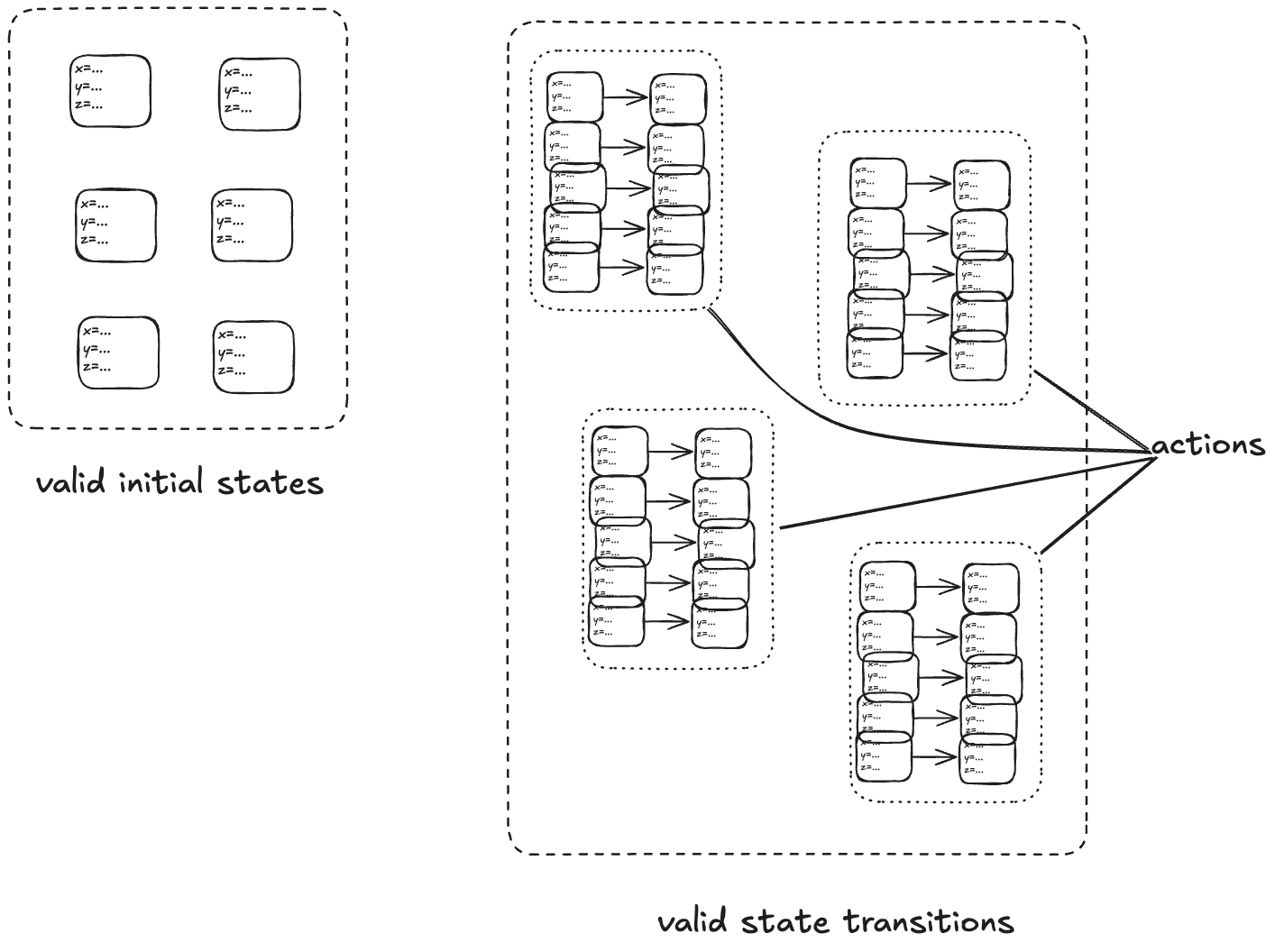
The transition-axiom method uses a state-machine model to describe a system. You describe a system by describing:
The set of valid initial states
The set of valid state transitions
(Aside: I’m not covering the more advanced topic of livenessin this post).
A set of related state transitions is referred to as an action. We use actions in TLA+ to model the events we care about (e.g., calling a function, sending a message).
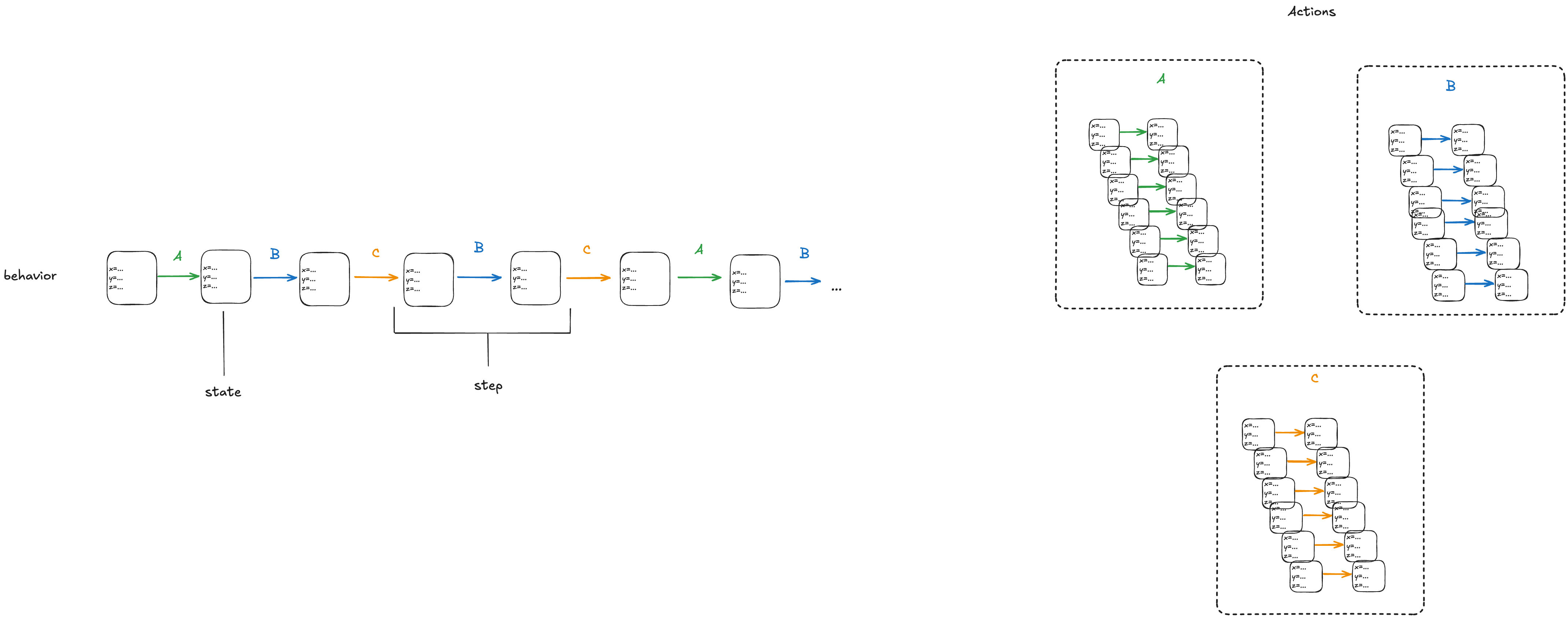
With a state-machine description, we can generate all sequences that start at one of the initial states and transition according to the allowed transitions. A sequence of states is called a behavior. A pair of successive states is called a step.
Each step in a behavior must be a member of one of the actions. In the diagram above, we would call the first step an A-step because it is a step that is a member of the A action.
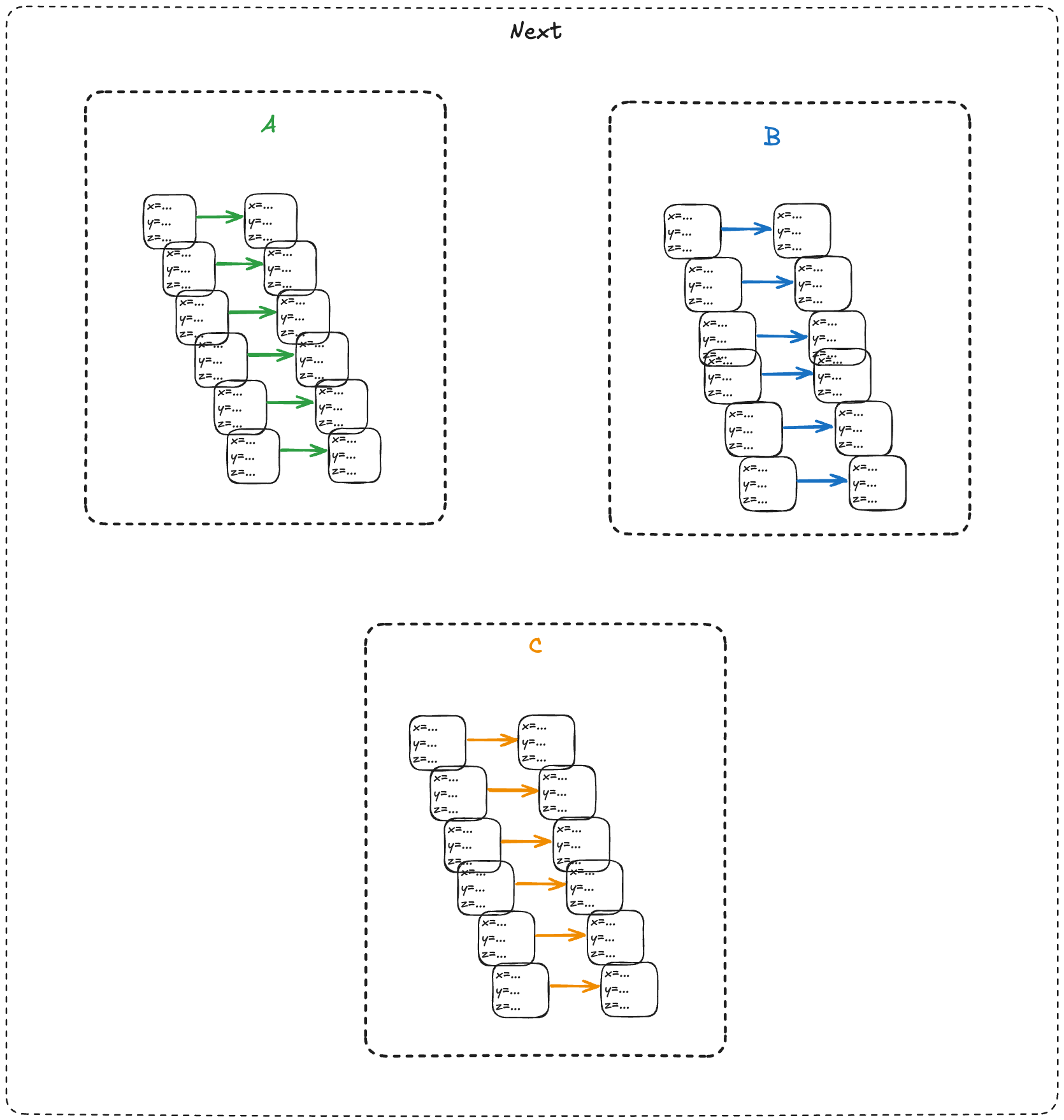
We refer to the set that includes all of the actions as the next-state action, which is typically called Next in TLA+ specifications.
In the example above, we would say that A, B, C are sub-actions of the Next action.
We call the entire state-machine description a specification: it defines the set of all allowed behaviors.
To make things concrete, let’s start with a simple example: a counter.
You think distributed systems is about trying to accomplish complex tasks, and then you read the literature and it's like "consider the problem of incrementing a counter", and it turns out that distributed systems is about how the simplest tasks become mind-bogglingly complex. https://t.co/4O2jfgfGQV
— @norootcause@hachyderm.io on mastodon (@norootcause) May 21, 2020
Modeling a counter with TLA+
Consider a counter abstract data type, that has only two operations:
inc – increment the counter
get – return the current value of the counter
reset – return the value of the counter to zero
Here’s an example execution history.
inc()
inc()
get() → 2
get() → 2
reset()
get() → 0
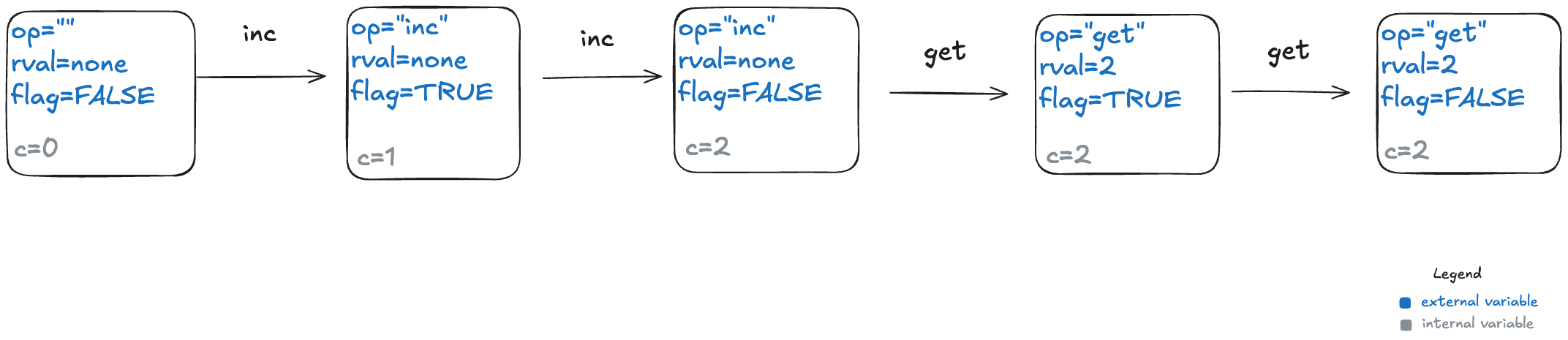
To model this counter in TLA+, we need to model the different operation types (inc, get, reset). We also need to model the return value for the get operation. I’ll model the operation with a state variable named op, and the return value with a state variable named rval.
But there’s one more thing we need to add to our model. In a state-machine model, we model an operation using one or more state transitions (steps) where at least one variable in the state changes. This is because all TLA+ models must allow what are called stuttering steps, where you have a state transition where none of the variables change.
This means we need to distinguish between two consecutive inc operations versus an inc operation followed by a stuttering step where nothing happens.
To do that, I’ll add a third variable to my model, which I’ll unimaginatively call flag. It’s a boolean variable, which I will toggle every time an operation happens. To sum up, my three state variables are:
op – the operation (“inc”, “get”, “reset”), which I’ll initialize to “” (empty string) in the first state
rval – the return value for a get operation. It will be a special value called none for all of the other operations
flag – a boolean that toggles on every (non-stuttering) state transition.
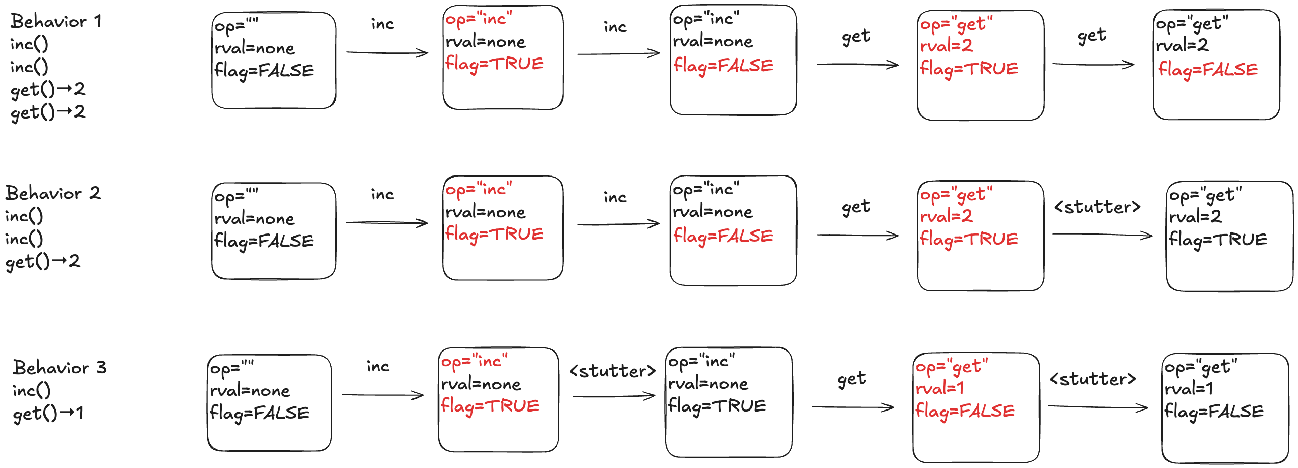
Below is a depiction of an execution history and how this would be modeled as a behavior at TLA+. The text in red indicated which variable changed in the transition. As mentioned above, every transition associated with an operation must have at least one variable that changes value.
Here’s a visual depiction of an execution history. Note how each event in the history is modeled as a step (pair of states) where at least one variable changes.
To illustrate why we need the extra variables, consider the following three behaviors.
In behavior 1, there are no stuttering steps. In behavior 2, the last step is a stuttering step, so there is only one “get” invocation. In behavior 3, there are two stuttering steps.
The internal variables
Our model of a counter so far has defined the external variables, which are the only variables that we really care about as the consumer of a specification. If you gave me a set of all of the valid behaviors for a queue, where behaviors were described using only these external behaviors, that’s all I need to understand how a queue behaves.
However, the external variables aren’t sufficient for the producer of a specification to actually generate the set of valid behaviors. This is because we need to keep track of some additional state information: how many increments there have been since the last reset. This type of variable is known as an internal state variable. I’m going to call this particular internal state variable c.
Here’s behavior 1, with different color codings for the external and internal variables.
The actions
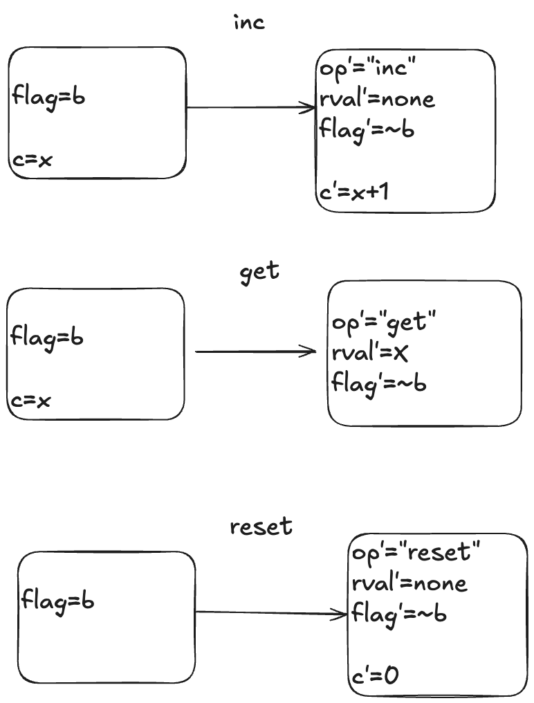
Here is a visual depiction of the permitted state transitions. Recall the set of permitted state transitions is called an action. For our counter, there are three actions, which corresponds to the three different operations we model: inc, get, and reset.
Each transition is depicted as two boxes with variables in it. The left-hand box shows the values of the variables before the state transition, and the right-hand box shows the values of the variables after the state transition. By convention we add a prime (‘) to the variables to refer to their values after the state transition.
While the diagram depicts three actions, each action describes a set of allowed state transitions. As an example, here are two different state transitions that are both members of the inc set of permitted transitions.
[flag=TRUE, c=5] → [flag=FALSE, c=6]
[flag=TRUE, c=8]→ [flag=FALSE, c=9]
In TLA+ terminology, we call these two steps inc steps. Remember: in TLA+, all of the action is in the actions. We use actions (sets of permitted state transitions) to model the events that we care about.
Modeling a queue with TLA+
We’ll move on to our second example, which will form the basis for the rest of this post: a queue. A queue supports two operations, which I’ll call enq (for enqueue) and deq (for dequeue).
Modeling execution histories as behaviors
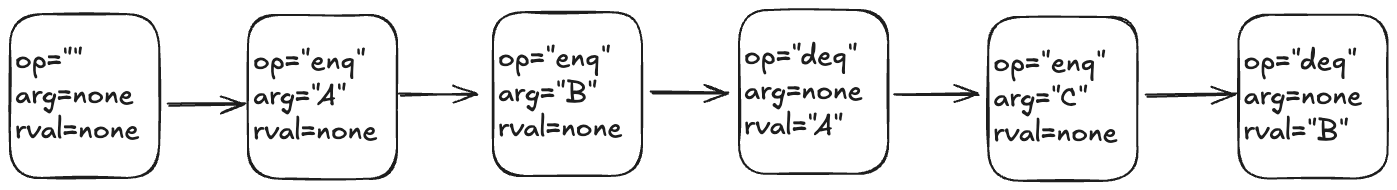
Recall our example of a valid execution history for a queue:
enq("A")
enq("B")
deq() → "A"
enq("C")
deq() → "B"
We now have to model argument passing, since the enq operation takes an argument.
Here’s one way to model this execution history as a TLA+ behavior.
My model uses three state variables:
op – identifies which operation is being invoked (enq or deq)
arg – the argument being passed in the case of the enq operation
rval – the return value in the case of the deq operatoin
TLA+ requires that we specify a value for every variable in every state, which means we need to specify a value for arg even for the deq operation, which doesn’t have an argument, and a value for rval for the enq operation, which doesn’t return a value. I defined a special value called none for this case.
In the first state, when the queue is empty, I chose to set op to the empty string (“”) and arg and rval to none.
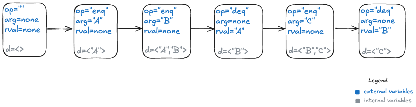
The internal variables
For a queue, we need to keep track all of the values that have previously been enqueued, as well as the order in which they were enqueued.
TLA+ has a type called a sequence which I’ll use to encode this information: a sequence is like a list in Python.
I’ll add a new variable which I’ll unimaginatively call d, for data. Here’s what that behavior looks like with the internal variable.
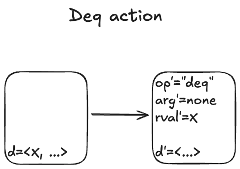
Modeling dequeues
Recall that our queue supports two operations: enqueue and dequeue. We’ll start with the dequeue operation. I modeled it with an action called Deq.
Here are some examples of state transitions that are permitted by the Deq action. We call these Deq steps.
I’m not going to write much TLA+ code in this post, but to give you a feel for it, here is how you would write the Deq action in TLA+ syntax:
The syntax of the first line might be a bit confusing if you’re not familiar with TLA+:
# is TLA+ for ≠
<<>> is TLA+ for the empty sequence.
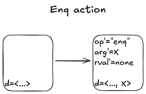
Modeling dequeues
Here’s what the Enq action looks like:
There’s non-determinism in this action: the value of arg’ can be any valid value that we are allowed to put onto the queue.
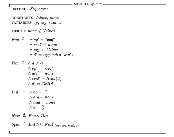
I’ll spend just a little time in this section to give you a sense of how you would use TLA+ to represent the simple queue model.
To describe the queue in TLA+, we define a set called Values that contains all of the valid values that could be enqueued, as well as a special constant named none that means “not a value”.
The complete description of our queue, its specification that describes all permitted behaviors, looks like this:
For completeness, here’s what the TLA+ specification looks like: (source in Queue.tla).
Init corresponds to our set of initial states, and Next corresponds to the next-state action, where the two sub-actions are Enq and Deq.
The last line, Spec, is the full specification. You can read this as: The initial state is chosen from the Init set of states, and every step is a Next step (every allowed state transition is a member of the set of state transitions defined by the Next action).
Modeling concurrency
In our queue model above, an enqueue or dequeue operation happens in one step (state transition). That’s fine for modeling sequential programs, but it’s not sufficient for modeling concurrent programs. In concurrent programs, the operations from two different threads can overlap in time.
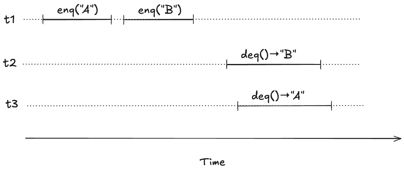
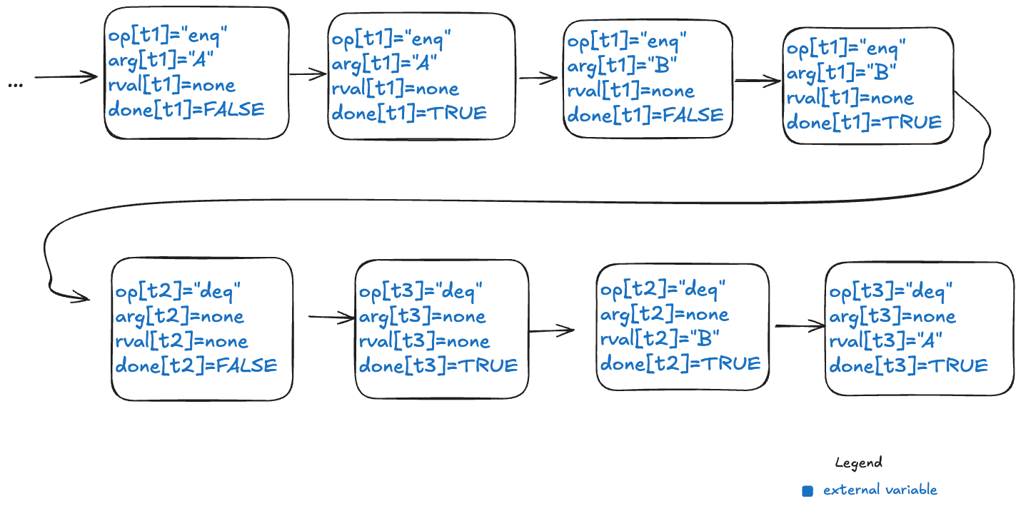
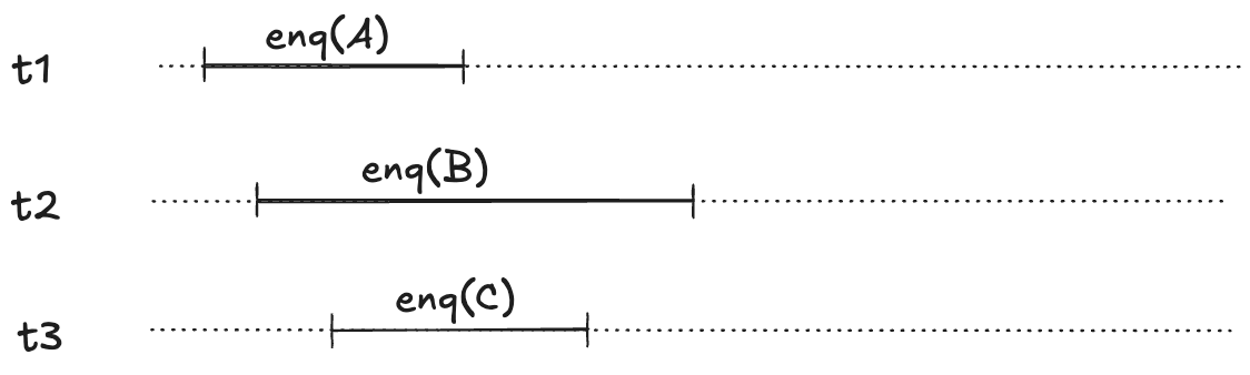
To illustrate, imagine a scenario where there are three threads, t1, t2, t3. First, t1 enqueues “A”, and “B”. Then, t2 and t3 both call dequeue, and those queries overlap in time.
We want to model concurrent executions using a state-machine model. The diagram above, shows the start and end time for each operation. But to model this behavior, we don’t actually care about the exact start and end times: rather, we only care about the relative order of the start and events.
We can model execution histories like the one above using state machines. We were previously modeling an operation in a single state transition (step). Now we will need to use two steps to model an operation: one to indicate when the operation starts and the other to indicate when the operate ends.
Because each thread acts independently, we need to model variables that are local to threads. And, in fact, all externally visible variables are scoped to threads, because each operation always happens in the context of a particular thread. We do this by changing the variables to be functions where the domain is a thread id. For example, where we previously had op=”enq” where op was always a string, now op is a function that takes a thread id as an argument. Now we would have op[t1]=”enq” where t1 is a thread id. (Functions in TLA+ use square brackets instead of round ones. you can think of these function variables as acting like dictionaries)
Here’s an example of a behavior that models the above execution history, showing only the external variables. Note that this behavior only shows the values that change in a state.
Note the following changes from the previous behaviors.
There is a boolean flag, done, which indicates when the operation is complete.
The variables are all scoped to a specific thread.
But what about the internal variable d?
Linearizability as correctness condition for concurrency
We know what it means for a sequential queue to be correct. But what do we want to consider correct when operations can overlap? We need to decide what it means for an execution history of a queue to be correct in the face of overlapping operations. This is where linearizability comes in. From the abstract of the Herlihy and Wing paper:
Linearizability provides the illusion that each operation applied by concurrent processes takes effect instantaneously at some point between its invocation and its response, implying that the meaning of a concurrent object’s operations can be given by pre- and post-conditions.
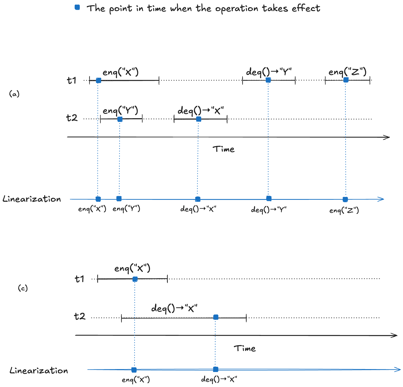
For our queue example, we say our queue is linearizable if, for every history where there are overlapping operations, we can identify a point in time between the start and end of the operation where the operation instantaneously “takes effect”, giving us a sequential execution history that is a correct execution history for a serial queue. This is a called a linearization. If every execution history for our queue has a linearization, then we say that our queue is linearizable.
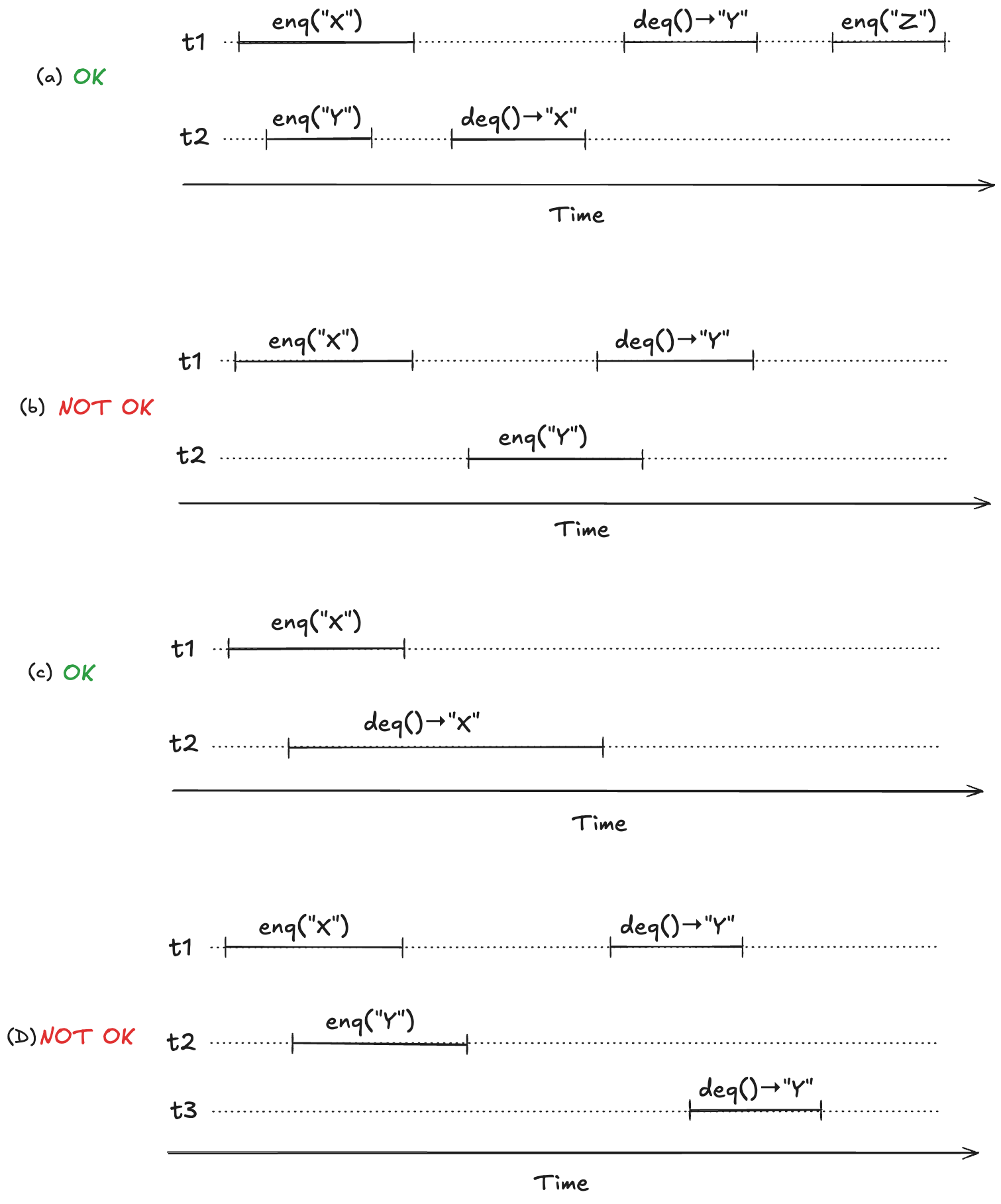
To make this concrete, consider the following four observed execution histories of a queue, labeled (a), (b), (c), (d), adapted from Fig. 1 of the Herlihy and Wing linearizable paper. Two of these histories are linearizable (they are labeled “OK”), and two are not (labeled “NOT OK”).
For (a) and (c), we can identify points in time during the operation where it appears as if the operation has instantaneously taken effect.
We now have a strict ordering of operations because there is no overlap, so we can write it as a sequential execution history. When the resulting sequential execution history is valid, it is called a linearization:
To repeat from the last section, a data structure is linearizable if, for every operation that executes on the data structure, we can identify a point in time between the start and the end of the operation where the operation takes effect.
We can model a linearizable queue by modeling each operation (enqueue/dequeue) as three actions:
Start (invocation) of operation
When the operation takes effect
End (return) of operation
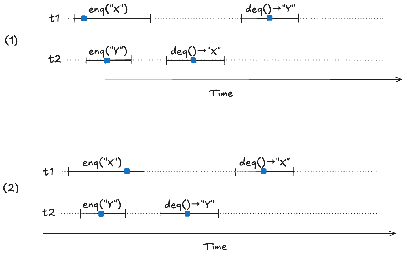
Our model needs to permit all possible linearizations. For example, consider the following two linearizable histories. Note how the start/end timings of the operations are identical in both cases, but the return values are different.
In (1) the first deq operation returns “X”, and in (2) the first deq operation “returns Y”. Yet they are both valid histories. The difference between the two is the order in which the enq operations take effect. In (1), enq(“X”) takes effect before enq(“Y”), and in (2), enq(“Y”) takes effect before enq(“X”). Here are the two linearizations:
Our TLA+ model of a linearizable queue will need to be able to model the relative order of when these operations take effect. This is where the internal variables come into play in our model: “taking effect” will mean updating internal variables of our model.
We need an additional variable to indicate whether the internal state has been updated or not for the current operation. I will call this variable up (for “updated”). It starts off as false when the operation starts, and is set to true when the internal state variable (d) has been updated.
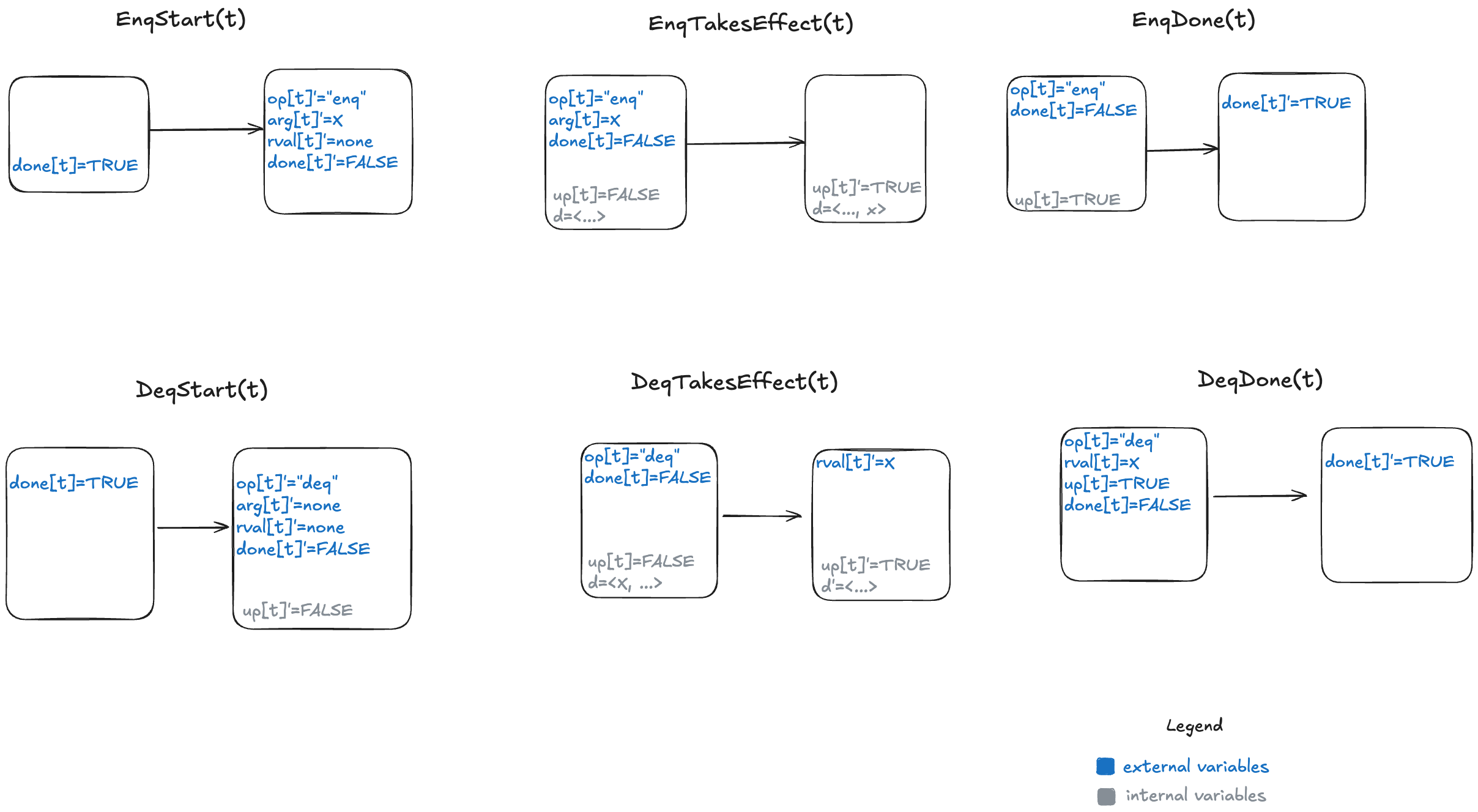
Here’s a visual representation of the permitted state transitions (actions). As before, the left bubble shows the values that must be true in the first state for the transition to happen, and the second bubble shows which variables change.
Since we now have to deal with multiple threads, we parameterize our action by thread id (t). You can see the TLA+ model here: LinearizableQueue.tla.
We now have a specification for a linearizable queue, which is a description of all valid behaviors. We can use this to verify that a specific queue implementation is linearizable. To demonstrate, let’s shift gears and talk about an example of an implementation.
An example queue implementation
Let’s consider an implementation of a queue that:
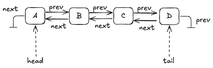
Stores the data in a doubly-linked list
Uses a lock to protect the list
A queue with four entries looks like this:
Here’s an implementation of this queue in Python that I whipped up. I call it an “LLLQueue” for “locked-linked-list queue”. I believe that my LLLQueue is linearizable, and I’d like to verify this.
One way is to use TLA+ to build a specification of my LLLQueue, and then prove that every behavior of my LLLQueue is also a behavior of the LinearizableQueue specification. The way we do this is in TLA+ is by a technique called refinement mappings.
But, first, let’s model the LLLQueue in TLA+.
Modeling the LLLQueue in TLA+ (PlusCal)
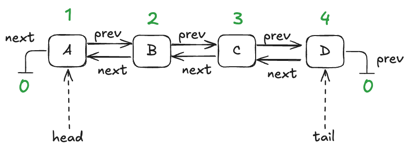
In a traditional program, a node would be associated with a pointer or reference. I’m going to use numerical IDs for each node, starting with 1. I’ll use the value of 0 as a sentinel value meaning null.
We’ll model this with three functions:
vals – maps node id to the value stored in the node
prev – maps node id to the previous node id in the list
next – maps node id to the next node id in the list
Here are these functions in table form for the queue shown above:
node id
vals
1
A
2
B
3
C
4
D
The vals function
node id
prev
1
2
2
3
3
4
4
0 (null)
The prev function
node id
next
1
0 (null)
2
1
3
2
4
3
The next function
It’s easier for me to use PlusCal to model an LLLQueue than to do it directly in TLA+. PlusCal is a language for specifying algorithms that can be automatically translated to a TLA+ specification.
It would take too much space to describe the full PlusCal model and how it translates, but I’ll try to give a flavor of it. As a reminder, here’s the implementation of the enqueue method in my Python implementation.
Here’s what my PlusCal model looks like for the enqueue operation:
procedure enqueue(val)
variable new_tail;
begin
E1: acquire(lock);
E2: with n \in AllPossibleNodes \ nodes do
        Node(n, val, tail);
        new_tail := n;
    end with;
E3: if IsEmpty then
        head := new_tail;
    else
        prev[tail] := new_tail;
    end if;
    tail := new_tail;
E4: release(lock);
E5: return;
end procedure;
Note the labels (E1, E2, E3, E4, E5) here. The translator turns those labels into TLA+ actions (state transitions permitted by the spec). In my model, an enqueue operation is implemented by five actions.
Refinement mappings
One of the use cases for formal methods is to verify that a (low-level) implementation conforms to a (higher-level) specification. In TLA+, all specs are sets of behaviors, so the way we do this is that we:
create a high-level specification that models the desired behavior of the system
create a lower-level specification that captures some implementation details of interest
show that every behavior of the low-level specification is among the set of behaviors of the higher-level specification, considering only the externally visible variables
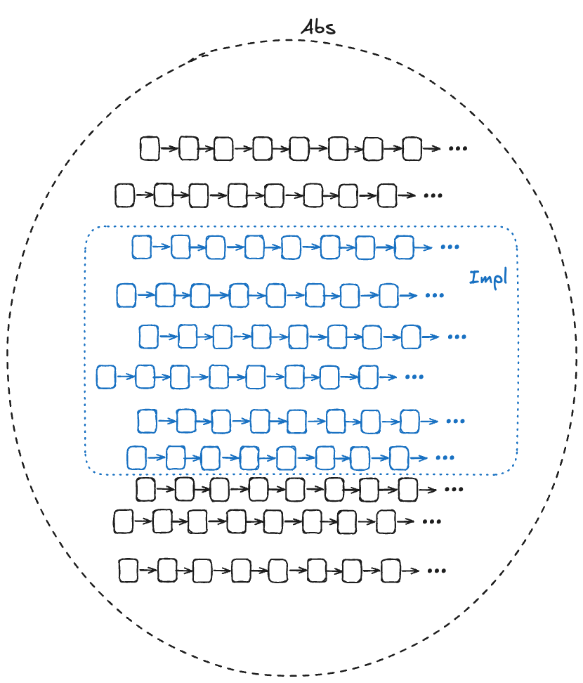
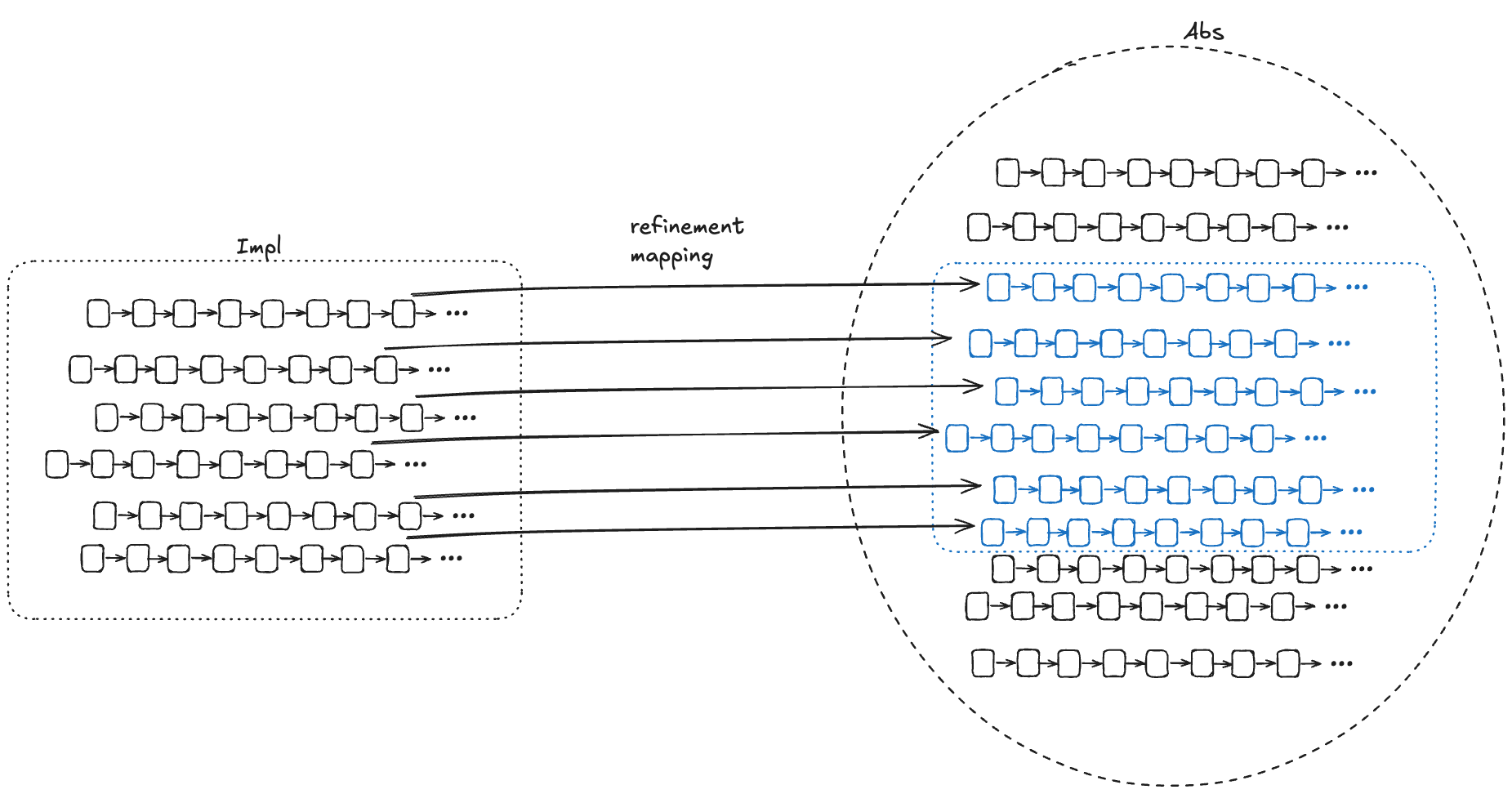
In the diagram below, Abs (for abstract) represents the set of valid (externally visible) behaviors of a high-level specification, and Impl (for implementation) represents the set of valid (externally visible) behaviors for a low-level specification. For Impl to implement Abs, the Impl behaviors must be a subset of the Abs behaviors.
We want to be able to prove that Impl implements Abs. In other words, we want to be able to prove that every externally visible behavior in Impl is also an externally visible behavior in Abs.
We want to be able to find a corresponding Abs behavior for every Impl behavior
One approach is to do this by construction: if we can take any behavior in Impl and construct a behavior in Abs with the same externally visible values, then we have proved that Impl implements Abs.
To prove that S1 implements S2, it suffices to prove that if S1 allows the behavior <<(e0,z0), (e1, z1), (e2, z2), …>>
where [ei is a state of the externally visible component and] the zi are internal states, then there exists internal states yi such that S2 allows <<(e0,y0), (e1, y1), (e2, y2), … >>
For each behavior B1 in Impl, if we can find values for internal variables in a behavior of Abs, B2, where the external variables of B2 match the external variables of B1, then that’s sufficient to prove that Impl implements Abs.
To show that Impl implements Abs, we need to find a refinement mapping, which is a function that will map every behavior in Impl to a behavior in Abs.
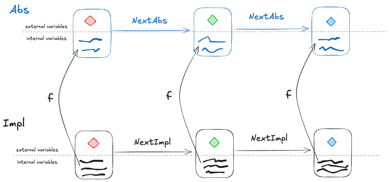
A refinement mapping takes a state in an Impl behavior as input and maps to an Abs state, such that:
the external variables are the same in both the Impl state and the Abs state
if a pair of states is a permitted Impl state transition, then the corresponding mapped pair of states must be a permitted Abs state transition
Or, to reword statement 2: if NextImpl is the next-state action for Impl (i.e., the set of allowed state transitions for Impl), and NextAbs is the next-state action for Abs, then under the refinement mapping, every NextImpl-step must map to a NextAbs step.
(Note: this technically isn’t completely correct, we’ll see why in the next section).
Example: our LLLQueue
We want to verify that our Python queue implementation is linearizable. We’ve modeled our Python queue in TLA+ as LLLQueue, and to prove that it’s linearizable, we need to show that a refinement mapping exists between the LLLQueue spec and the LinearizableQueue spec. This means we need to show that there’s a mapping from LLLQueue’s internal variables to LinearizableQueue’s internal variables.
We need to define the internal variables in LinearizableQueue (up, d) in terms of the variables in LLLQueue (nodes, vals, next, prev, head, tail, lock, new_tail, empty, pc, stack) in such a way that all LLLQueue behaviors are also LinearizableQueue behaviors under the mapping.
Internal variable: d
The internal variable d in LinearizableQueue is a sequence which contains the values of the queue, where the first element of the sequence is the head of the queue.
Looking back at our example LLLQueue queue:
We need a mapping that, for this example, results in: d =〈A,B,C,D 〉
I defined a recursive operator that I named Data such that when you call Data(head), it evaluates to a sequence with the values of the queue.
Internal variable: up
The variable up is a boolean flag that flips from false to true after the value has been added to the queue.
In our LLLQueue model, the new node gets added to the tail by the action E3. In PlusCal models, there’s a variable named pc (program counter) that records the current execution state of the program. You can think of pc like a breakpoint that points to the action that will be executed on the next step of the program. We want up to be true after action E3. You can see how the up mapping is defined at the bottom of the LLLQueue.tla file.
Refinement mapping and stuttering
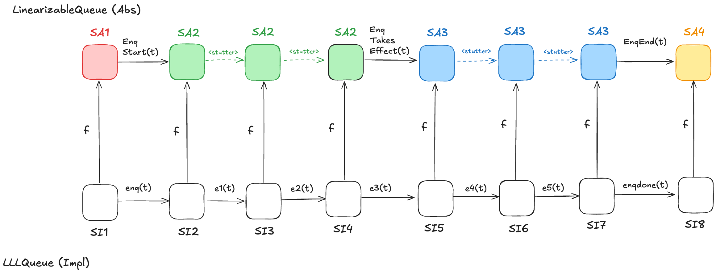
Let’s consider a behavior of the LLLQueue spec that enqueues a single value onto the queue, with a refinement mapping to the LinearizableQueue spec:
In the LinearizableQueue spec, an enqueue operation is implemented by three actions:
EnqStart
EnqTakesEffect
EnqEnd
In the LLLQueue spec, an enqueue operation is implemented by seven actions: enq, e1, …, e5, enqdone. That means that the LLLQueue enqueue behavior involves eight distinct states, where the corresponding LinearizableQueue behavior involves only four distinct states. Sometimes, different LLLQueue states map to the same LinearizableQueue state. In the figure above, SI2,SI3,SI4 all map to SA2, and SI5,SI6,SI7 all map to SA3. I’ve color-coded the states in the LinearizableQueue behavior such that states that have the same color are identical.
As a result, some state transitions in the refinement mapping are not LinearizableQueue actions, but are instead transitions where none of the variables change at all. These are called stuttering steps. In TLA+, stuttering steps are always permitted in all behaviors.
A problem with refinement mappings: the Herlihy and Wing queue
The last section of the Herlihy and Wing paper describes how to prove that a concurrent data structure’s operations are linearizable. In the process, the authors also point out a problem with refinement mappings. They illustrate the problem using a particular queue implementation, which we’ll call the “Herlihy & Wing queue”, or H&W Queue for short.
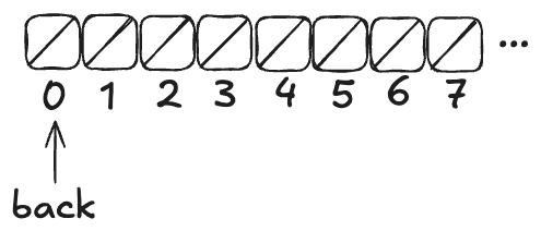
Imagine an array of infinite length, where all of the values are initially null. There’s a variable named back which points to the next available free spot in the queue.
Enqueueing
To enqueue a value onto the Herlihy & Wing queue involves two steps:
Increment the back variable
Write the value into the spot where the back variable pointed before being incremented .
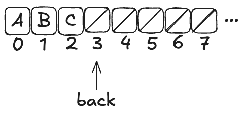
Here’s what the queue looks like after three values (A,B,C) have been enqueued:
Note how back always points to the next free spot.
Dequeueing
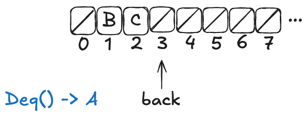
To dequeue, you start at index 0, and then you sweep through the array, looking for the first non-null value. Then you atomically copy that value out of the array and set the array element to null.
Here’s what a dequeue operation on the queue above would look like:
The Deq operation returned A, and the first element in the array has been set to null.
If you were to enqueue another value (say, D), the array would now look like this:
Note: the elements at the beginning of the queue that get set to null after a dequeue don’t get reclaimed. The authors note that this is inefficient, but the purpose of this queue is to illustrate a particular issue with refinement mappings, not to be a practical queue implementation.
H&W Queue pseudocode
Here’s the pseudocode for Herlihy & Wing queue, which I copied directly from the paper. The two operations are Enq (enqueue) and Deq (dequeue).
rep = record {back: int, items: array [item]}

Enq = proc (q: queue, x: item)
  i: int := INC(q.back) % Allocate a new slot
  STORE (q.items[i], x) % Fill it.
  end Enq

Deq = proc (q: queue) returns (item)
  while true do
    range: int := READ(q.back) - 1
    for i: int in 1 .. range do
      x: item := SWAP(q.items[i], null)
      if x ~= null then return(x) end
      end
    end
end Deq
This algorithm relies on the following atomic operations on shared variables:
INC – atomically increment a variable and return the pre-incremented value
STORE – atomically write an element into the array
READ – atomically read an element in the array (copy the value to a local variable)
SWAP – atomically write an element of an array and return the previous array value
H&W Queue implementation in C++
Here’s my attempt at implementing this queue using C++. I chose C++ because of its support for atomic types. C++’s atomic types support all four of the atomic operations required of the H&W queue.
Atomic operation
Description
C++ equivalent
INC
atomically increment a variable and return the pre-incremented value
My queue implementation stores pointers to objects of parameterized type T. Note the atomic types of the member variables. The back variable and elements of the items array need to be atomics because we will be invoking atomic operations on them.
template <typename T>
class Queue {
    atomic<int> back;
    atomic<T *> *items;

public:
    Queue(int sz) : back(0), items(new atomic<T *>[sz]) {}
    ~Queue() { delete[] items; }

    void enq(T *x);
    T *deq();
};

template<typename T>
void Queue<T>::enq(T *x) {
    int i = back.fetch_add(1);
    std::atomic_store(&items[i], x);
}

template<typename T>
T *Queue<T>::deq() {
    while (true) {
        int range = std::atomic_load(&back);
        for (int i = 0; i < range; ++i) {
            T *x = std::atomic_exchange(&items[i], nullptr);
            if (x != nullptr) return x;
        }
    }
}
We can write enq and deq to look more like idiomatic C++ by using the following atomic operators:
Using these operators, enq and deq look like this:
template<typename T>
void Queue<T>::enq(T *x) {
    int i = back++;
    items[i] = x;
}

template<typename T>
T *Queue<T>::deq() {
    while (true) {
        int range = back;
        for (int i = 0; i < range; ++i) {
            T *x = std::atomic_exchange(&items[i], nullptr);
            if (x != nullptr) return x;
        }
    }
}
Note that this is, indeed, a linearizable queue, even though it does not use mutual exclusion: tthere are no critical sections in the algorithm.
Modeling the H&W queue in TLA+ with PlusCal
The H&W queue is straightforward to model in PlusCal. If you’re interested in learning PlusCal, it’s actually a great example to use. See HWQueue.tla for my implementation.
Refinement mapping challenge: what’s the state of the queue?
Note how the enq method isn’t an atomic operation. Rather, it’s made up of two atomic operations:
Increment back
Store the element in the array
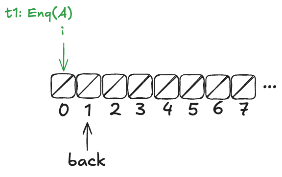
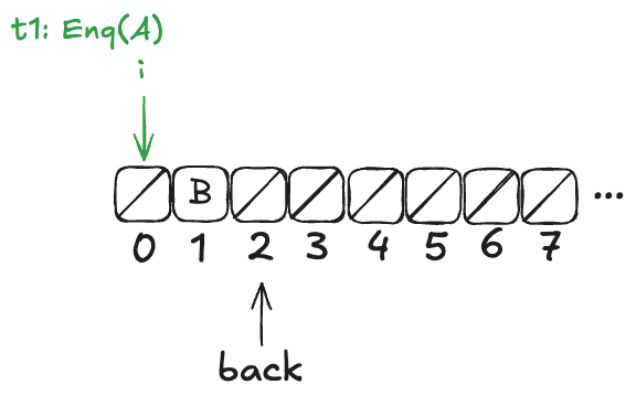
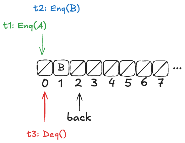
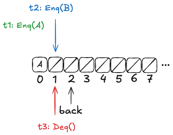
Now, imagine that a thread, t1, comes along, to enqueue a value to the queue. It starts off by incrementing back.
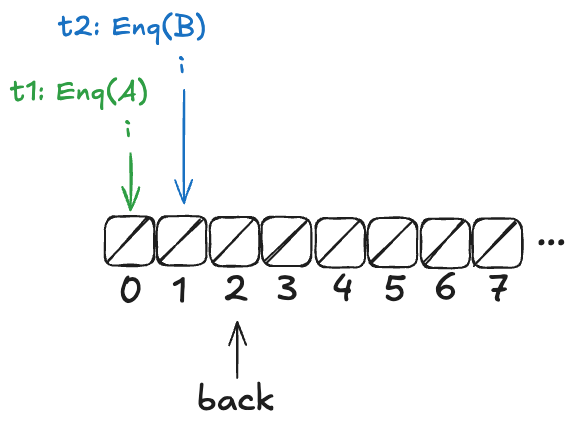
But before it can continue, a new thread, t2, gets scheduled, which also increments back:
t2 then completes the operation:
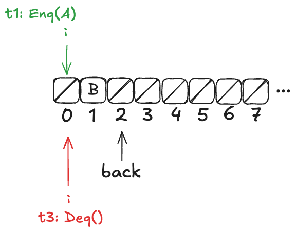
Finally, a new thread, t3, comes along that executes the dequeue operation:
Example state of the H&W queue
Now, here’s the question: What value will the pending Deq() operation return: A or B?
The answer: it depends on how the threads t1 and t3 will be scheduled. If t1 is scheduled first, it will write A to position 0, and then t3 will read it. On the other hand, if t3 is scheduled first, it will advance its i pointer to the next non-null value, which is position 1, and return B.
Recall back in the section “Modeling a queue with TLA+ > The internal variables” that our model for a linearizable queue had an internal variable, named d, that contained the elements of the queue in the order in which they had been enqueued.
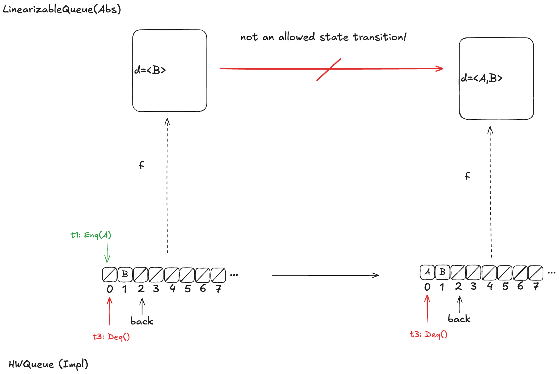
If we were to write a refinement mapping of this implementation to our linearizable specification, for the state above, we’d have to decide whether the mapping for the above state should be. The problem is that no such refinement mapping exists.
Here are the only options that make sense for the example above:
d =〈B〉
d =〈A,B〉
d =〈B,A〉
As a reminder, here are the valid state transitions for the LinearizableQueue spec.
Option 1: d =〈B〉
Let’s say we define our refinement mapping by using the populated elements of the queue. That would result in a mapping of d =〈B〉.
The problem is that if t1 gets scheduled first and adds value A to array position 0, then an element will be added to the head of d. But the only LinearizableQueue action that adds an element to d is EnqTakeEffect, which adds a value to the to the end of d. There is no LinearizableQueue action that allows prepending to d, so this cannot be a valid refinement mapping.
Option 2: d =〈A,B〉
Let’s say we had chosen instead a refinement mapping of d =〈A,B〉for the state above. In that case, if t3 gets scheduled first, then it will result in a value being removed from the end of d, which is not one of the actions of the LinearizableQueueSpec, which means that this can’t be a valid refinement mapping either.
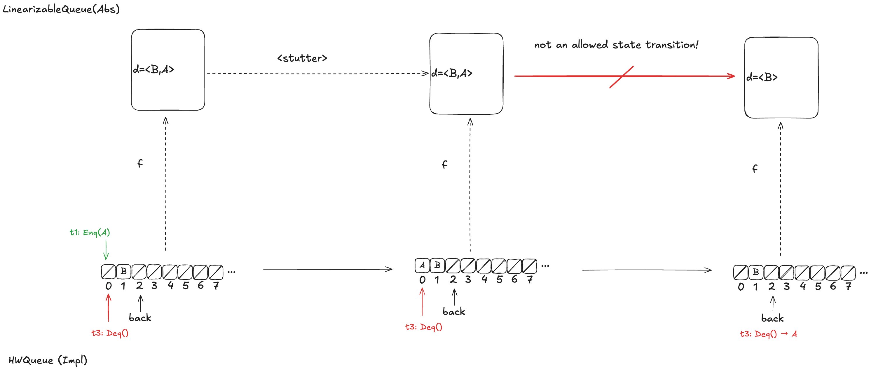
Option 3: d =〈B,A〉
Finally, assume we had chosen d =〈B,A〉as our refinement mapping. Then, if t1 gets scheduled first, and then t3, we will end up with a state transition that removes an element from the end of d, which is not a LinearizableQueue action.
Whichever refinement mapping we choose, it is possible that the resulting behavior will violate the LinearizableQueue spec. This means that we can’t come up with a refinement mapping where every behavior of Impl maps to a valid behavior of Abs, even though Impl implements a linearizable queue!
What Lamport and others believed at the time was that this type of refinement mapping always existed if Impl did indeed implement Abs. With this counterexample, Herlihy & Wing demonstrated that this was not always the case.
Elements in H&W queue aren’t totally ordered
In a typical queue implementation, there is a total ordering of elements that have been enqueued. The odd thing about the Herlihy & Wing queue is that this isn’t the case.
If we look back at our example above:
If t1 is scheduled first, A is dequeued next. If t3 is scheduled first, B is dequeued next.
Either A or B might be dequeued next, depending on the ordering of t1 and t3. Here’s another example where the value dequeued next depends on the ordering of the threads t1 and t3.
If t2 is scheduled first, B is dequeued next. If t3 is scheduled first, A is dequeued next.
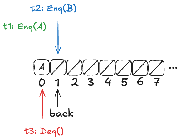
However, there are also scenarios where there is a clear ordering among values that have been added to the queue. Consider a case similar to the one above, except that t2 has not yet incremented the back variable:
In this configuration, A is guaranteed to be dequeued before B. More generally, if t1 writes A to the array before t2 increments the back variable, then A is guaranteed to be dequeued before B.
In the linearizability paper, Herlihy & Wing use a mapping approach where they identify a set of possible mappings rather than a single mapping.
Let’s think back to this scenario:
If t1 is scheduled first, A is dequeued next. If t3 is scheduled first, B is dequeued next.
In the scenario above, in the Herlihy and Wing approach, the mapping would be to the set of all possible values of queue.
queue ∈ {〈B〉,〈A,B〉, 〈B,A〉}
Lamport took a different approach to resolving this issue. He rescued the idea of refinement mappings by introducing a concept called prophecy variables
Prophecy
The Herlihy & Wing queue’s behavior is non-deterministic: we don’t know the order in which values will be dequeued, because it depends on the scheduling of the threads. But imagine if we know in advance the order in which the values were dequeued.
It turns out that if we can predict the order in which the values would be dequeued, then we can do a refinement mapping to the our LinearizableQueue model.
This is the idea behind prophecy variables: we predict certain values that we need for refinement mapping.
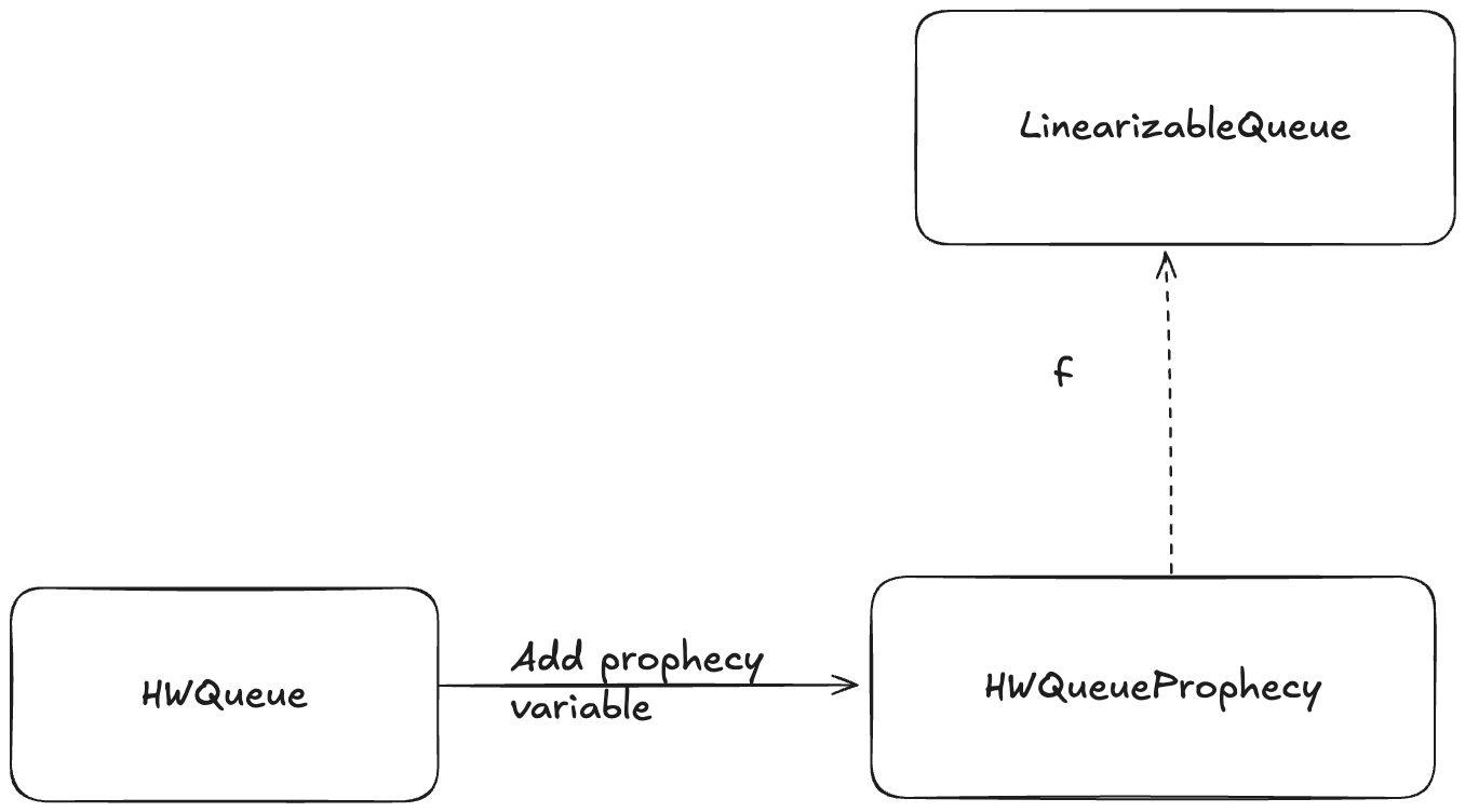
Adding a prophecy variable gives us another specification (one which has a new variable), and this is the specification where we can define a refinement mapping. For example, we add a prophecy to our HWQueue model and call the new model HWQueueProphecy.
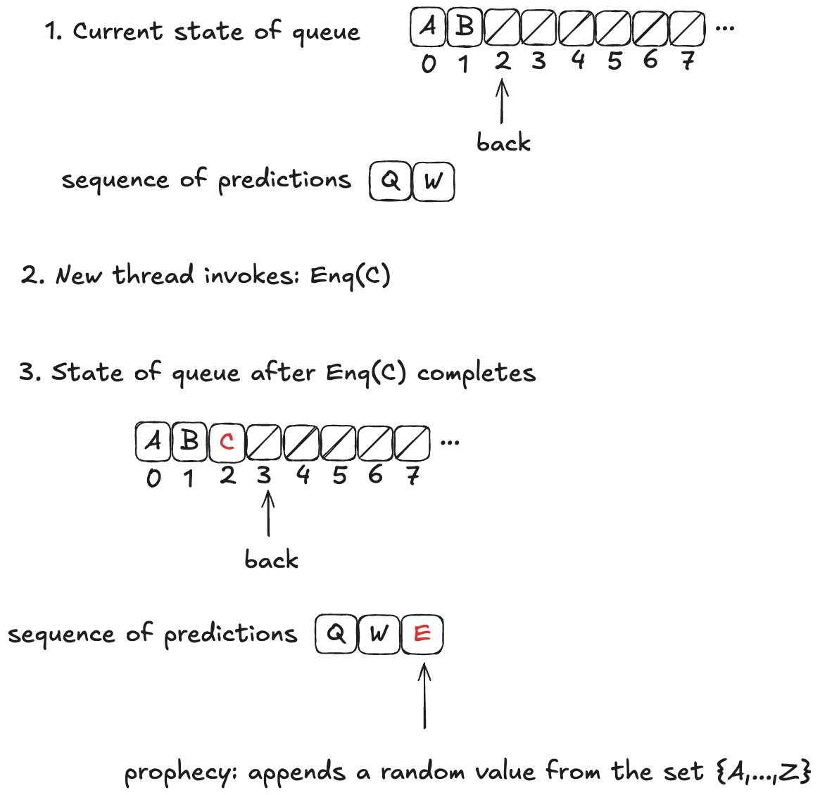
In HWQueueProphecy, we maintain a sequence of the predicted order in which values will be dequeued. Every time a thread invokes the enqueue operation, we add a new value to our sequence of predicted dequeue operations.
The predicted value is chosen at random from the set of all possible values: it is not necessarily related to either the value currently being enqueued or the current state of the queue.
Now, these predictions might not actually come true. In fact, they almost certainly won’t come true, because we’re much more likely to predict at least one value incorrectly. In the example above, the actual dequeueing order will be〈A,B,C〉, which is different from the predicted dequeueing order of〈Q,W,E〉
However, the refinement mapping will still work, even though the predictions will often be wrong, if we set things up correctly. We’ll tackle that next.
Prophecy requirements
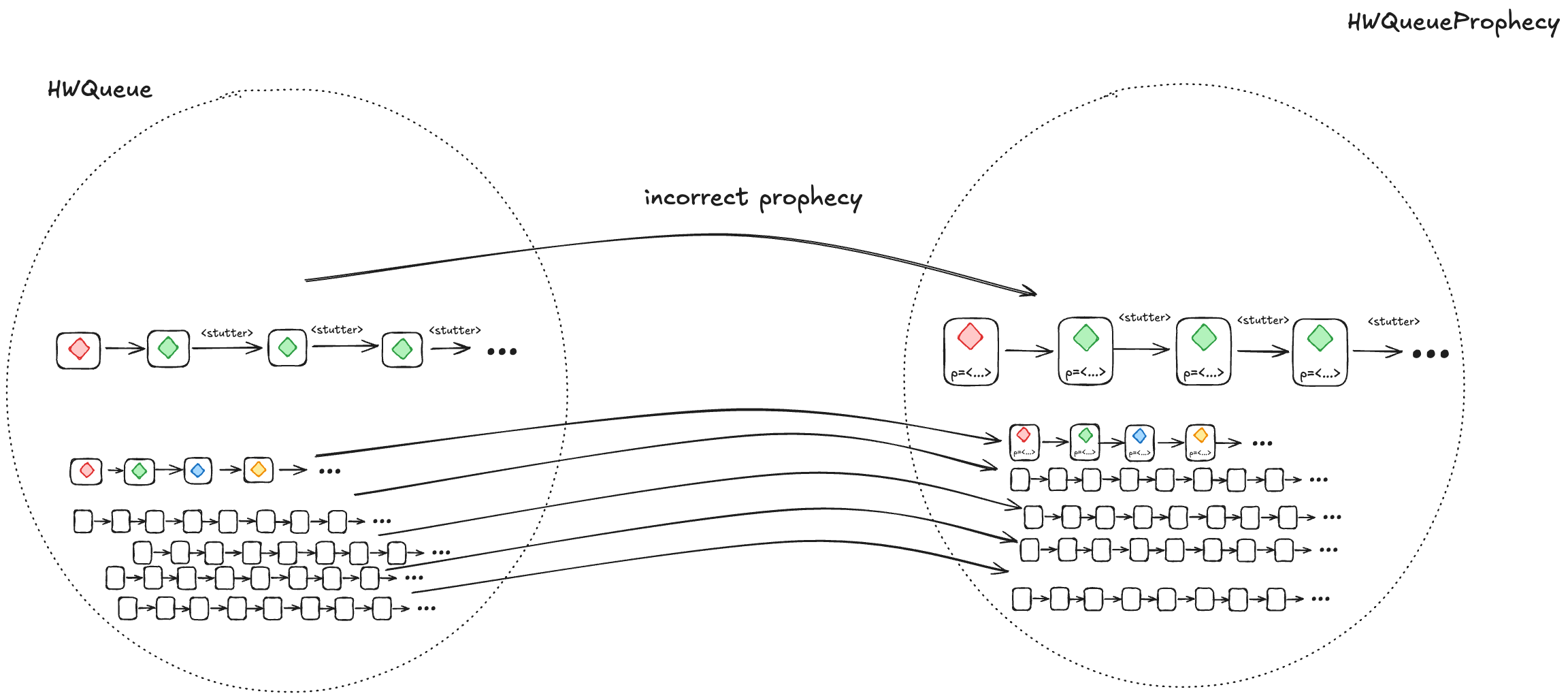
We want to show that HWQueue implements LinearizableQueue. But it’s only HWQueueProphecy that we can show implements LinearizableQueue using a refinement mapping.
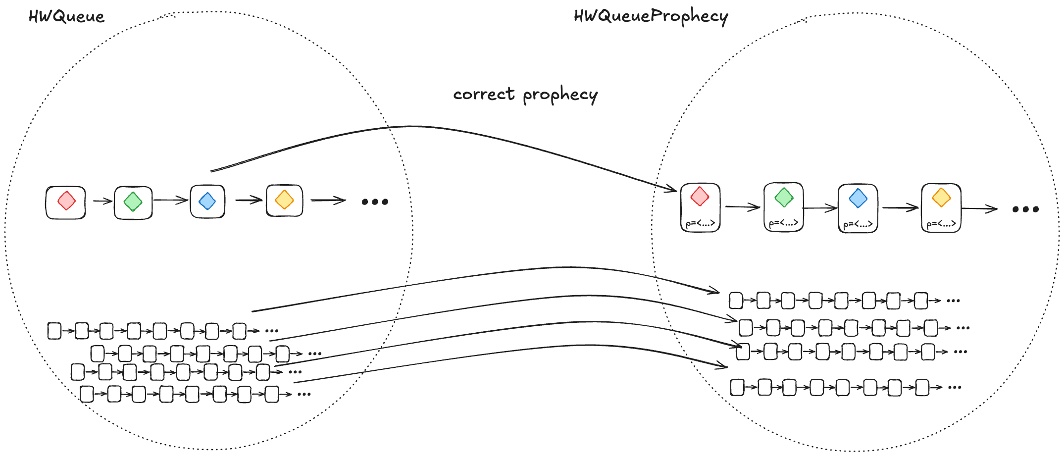
1. A correct prophecy must exist for every HWQueue behavior
Every behavior in HWQueue must have a corresponding behavior in HWQueueProphecy. That correspondence happens when the prophecy accurately predicts the dequeueing order.
This means that, for each behavior in HWQueue, there must be a behavior in HWQueueProphecy which is identical except that the HWQueueProphecy behaviors have an additional p variable with the prophecy.
To ensure that a correct prophecy always exists, we just make sure that we always predict from the set of all possible values.
In the case of HWQueueProphecy, we are always enqueueing values from the set {A,…,Z}, and so as long as we draw predictions from the set {A,…,Z}, we are guaranteed that the correct prediction is among the set we are predicting from.
2. Every HWQueueProphecybehaviorwith an incorrect prophecy must correspond to at least one HWQueue behavior
Most of the time, our predictions will be incorrect. We need to ensure that, when we prophesize incorrectly, the resulting behavior is still a valid HWQueue behavior, and is also still a valid LinearizableQueue behavior under refinement.
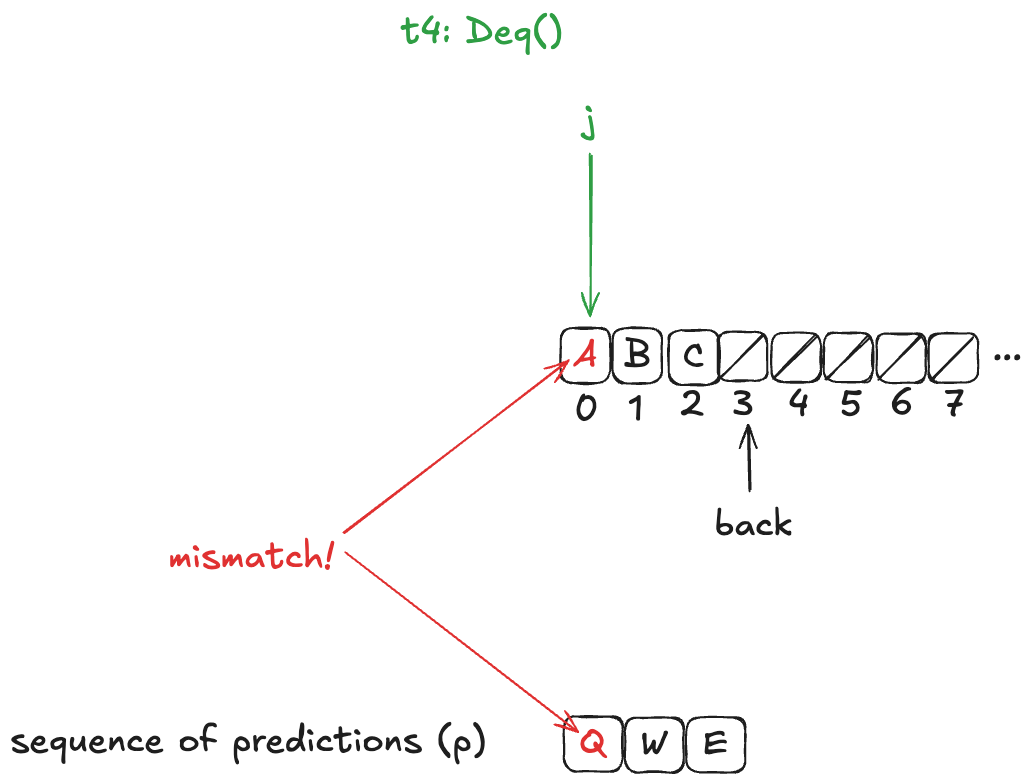
We do this by writing our HWQueueProphecy specification such that, if our prediction turns out to be incorrect (e.g., we predict A as the next value to be dequeued, and the next value that will actually be dequeued is B), we disallow the dequeue from happening.
In other words, we disallow state transitions that would violate our predictions.
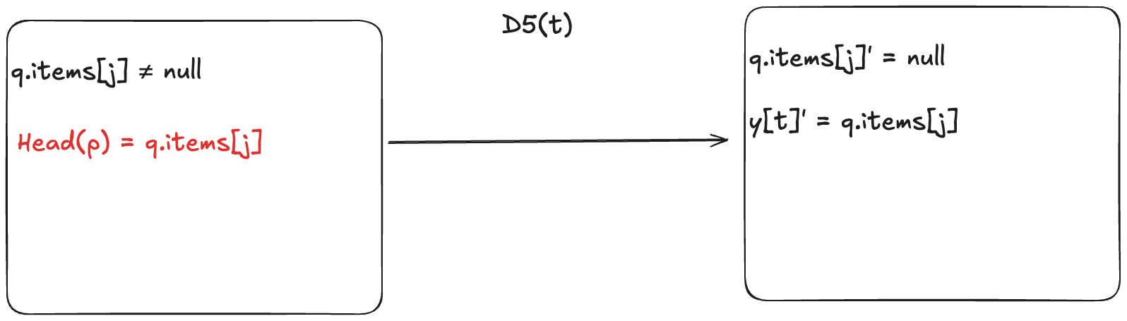
This means we add a new enabling condition to one of the dequeue actions. Now, for the dequeueing thread to remove the value from the array, it has to match the next value in the predicted sequence. In HWQueueProphecy, the name of the action that does this is D5, where t is id of the thread doing the dequeueing.
An incorrect prophecy blocks the dequeueing from actually happening. In the case of HWQueueProphecy, we can still enqueue values (since we don’t make any predictions on enqueue order, only dequeue order, so there’s nothing to block).
But let’s consider the more interesting case where an incorrect prophecy results in deadlock, where no actions are enabled anymore. This means that the only possible future steps in the behavior are stuttering steps, where the values never change.
When a prophecy is incorrect, it can result in deadlock, where all future steps are stuttering steps. These are still valid behaviors.
However, if we take a valid behavior of a specification, and we add stuttering steps, the resulting behavior is always also a valid behavior of the specification. So, the resulting behaviors are guaranteed to be in the set of valid HWQueue behaviors.
Using the prophecy to do the refinement mapping
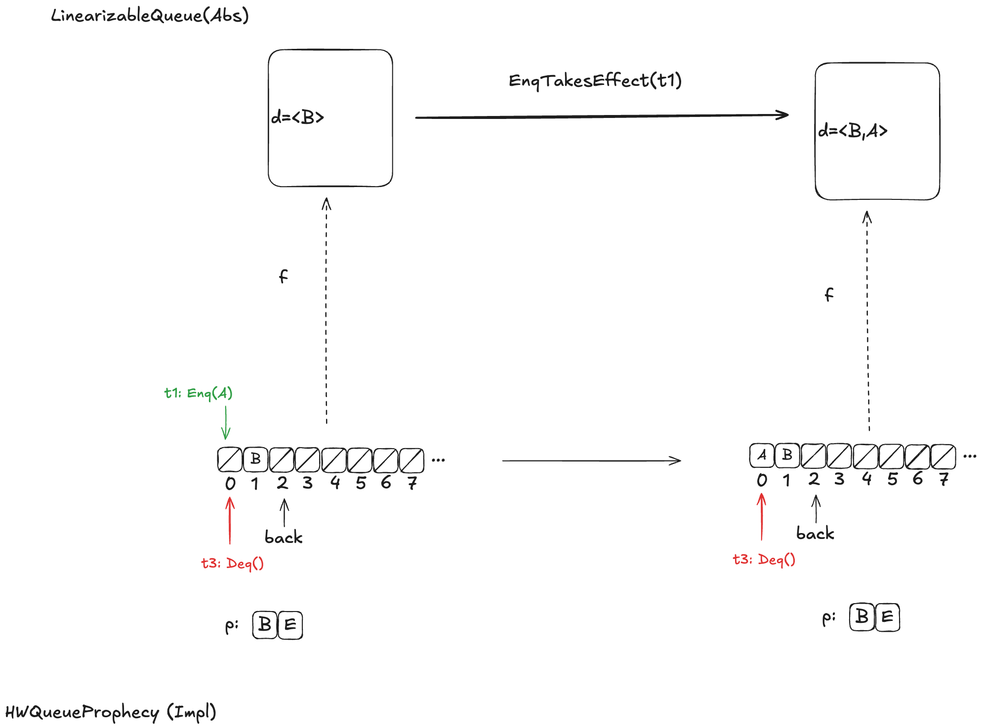
Let’s review what we were trying to accomplish here. We want to figure out a refinement mapping from HWQueueProphecy to LinearizableQueue such that every state transition satisfies the LinearizableQueue specification.
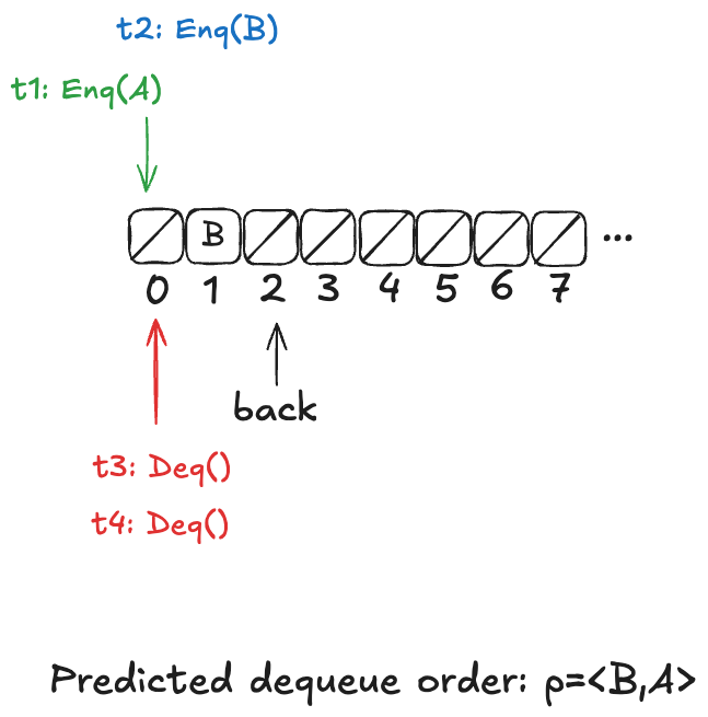
Here’s an example, where the value B has been enqueued, the value A is in the process of being enqueued, and no values have been dequeued yet.
Defining how to do this mapping is not obvious, and I’m not going to explain it here, as it would take up way too much space, and this post is already much too long. Instead, I will defer interested readers to section 6.5 of Lamport’s book A Science of Concurrent Programs, which describes how to do the mapping. See also my POFifopq.tla spec, which is my complete implementation of his description.
But I do want to show you something about it.
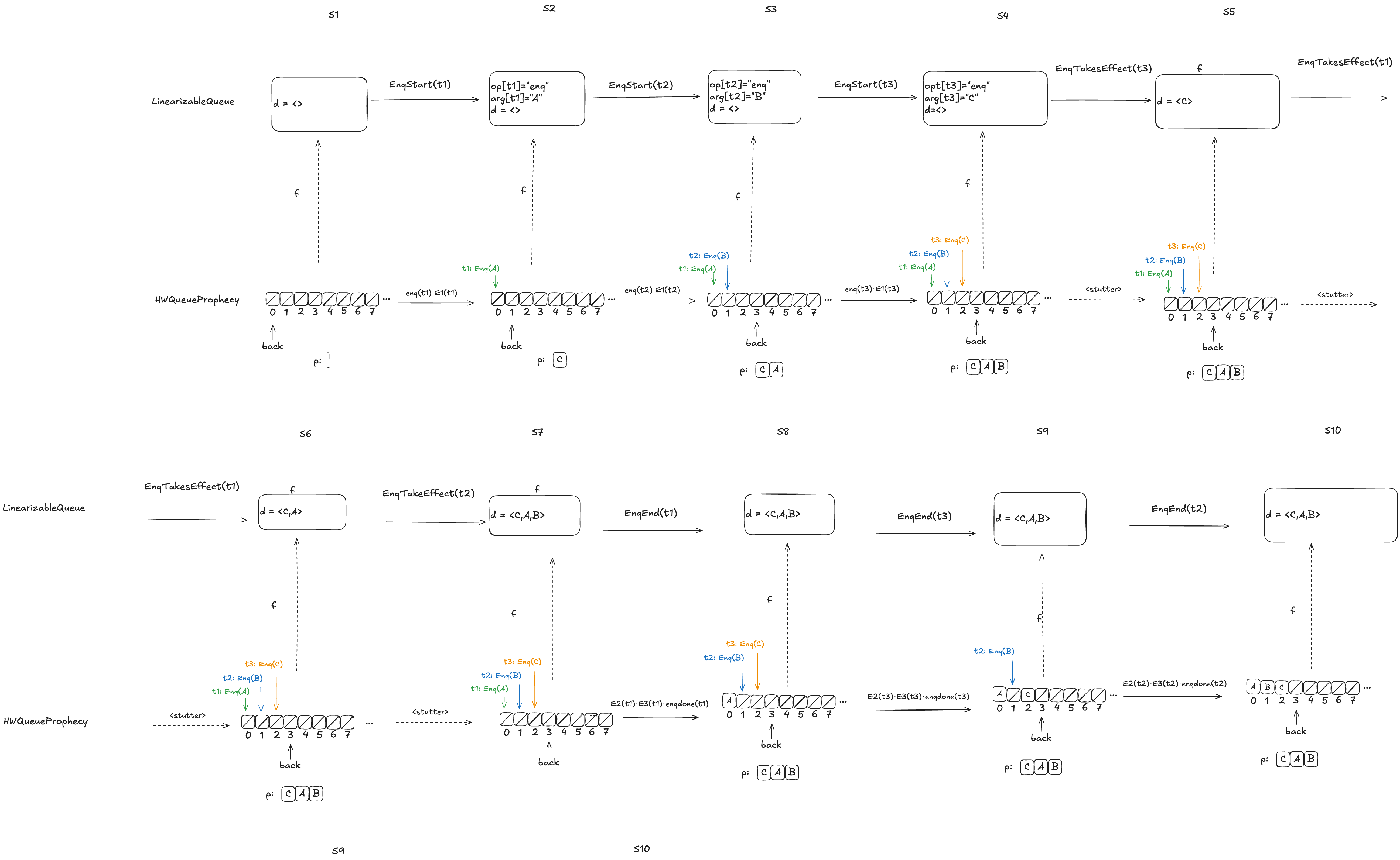
Enqueue example
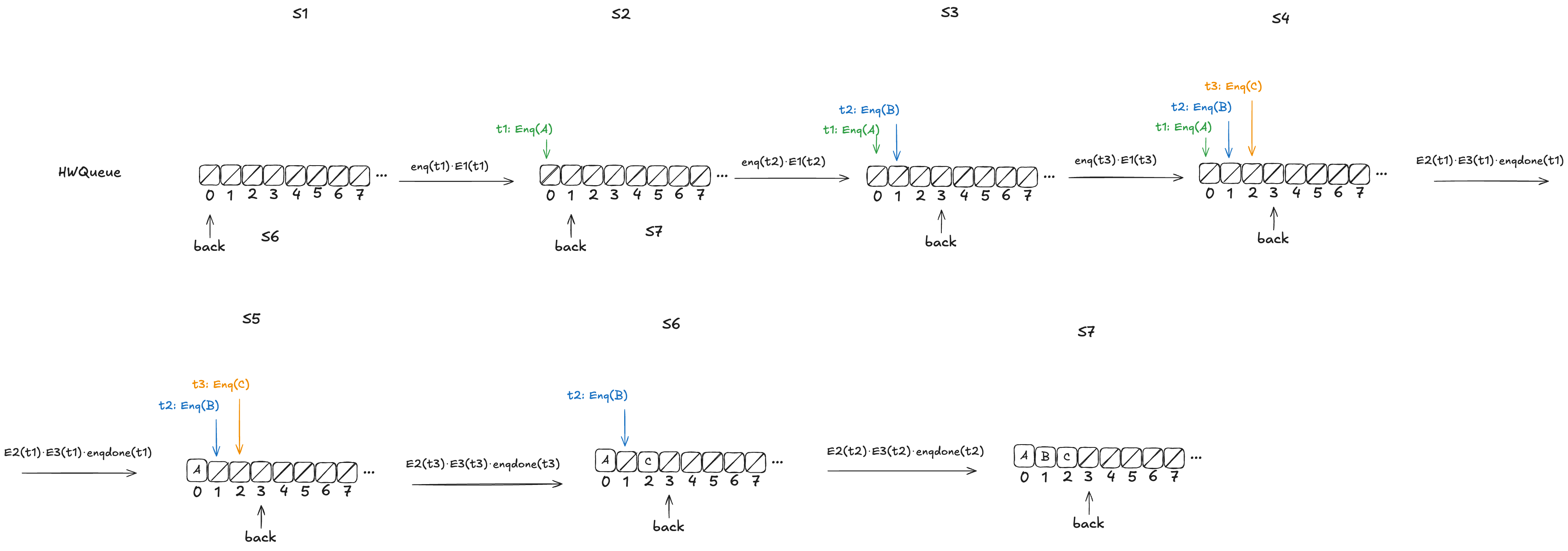
Let’s consider this HWQueue behavior, where we are concurrently enqueueing three values (A,B,C):
These enqueue operations all overlap each other, like this:
The refinement mapping will depend on the predictions.
Here’s an example where the predictions are consistent with the values being enqueued. Note how the state of the mapping ends up matching the predicted values.
Notice how in the final state (S10), the refinement mapping d=〈C,A,B〉is identical to the predicted dequeue ordering: p=〈C,A,B〉.
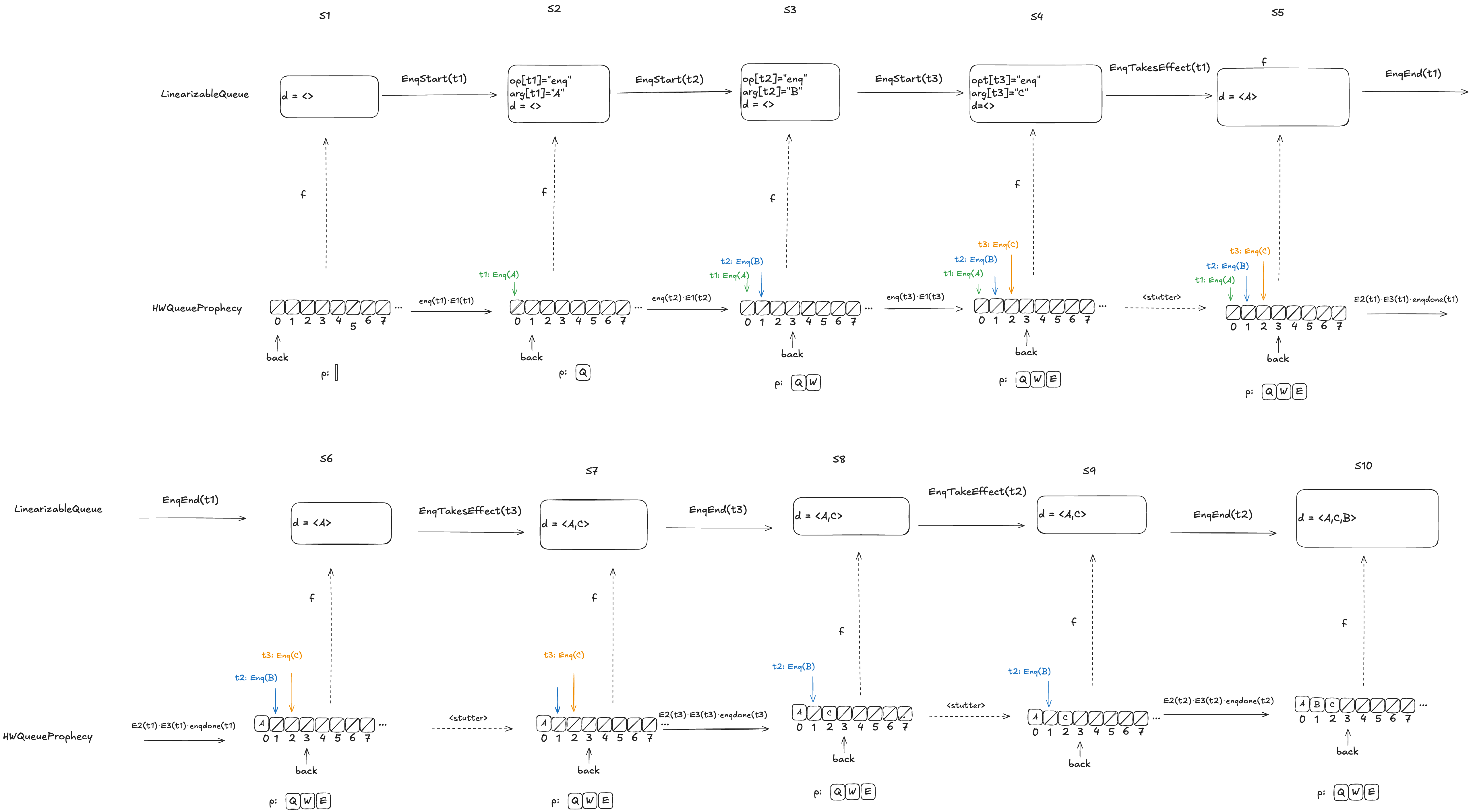
Here the predicted dequeue values p=〈Q,W,E〉can never be fulfilled, and the refinement mapping in this case, d=〈A,C,B〉matches the order in which overlapping enqueue operations complete.
The logic for determining the mapping varies depending on whether it is possible for the predictions to be fulfilled. For more details on this, see A Science of Concurrent Programs.
For the dequeueing case, if the value to be dequeued matches the first prediction in p, then we execute the dequeue and we remove the prediction from p. (We’ve already discussed the behavior if the value to be dequeued doesn’t match the prediction).
Coda
Phew! There was a lot of content in this post, including definitions and worked out examples. It took me a long time to grok a lot of this material, so I suspect that even an interested reader won’t fully absorb it on the first read. But if you got all of the way here, you’re probably interested enough in TLA+ that you’ll continue to read further on it. I personally find that it helps to have multiple explanations and examples, and I’ve tried to make an effort to present these concepts a little differently than other sources, so hopefully you’ll find it useful to come back here after reading elsewhere.
A Science of Concurrent Programs. Leslie Lamport. This is a self-published book on how to use TLA to model concurrent algorithms. This book documents how to use prophecy variables to implement the refinement mapping for the linearizable queue in the Herlihy and Wing paper.
Consistency Models. Linearizability is a consistency models, but there are multiple other ones. Kyle Kingsbury provides a good overview of the different models on his Jepsen site.
Yesterday, CrowdStrike released a Preliminary Post-Incident Review of the major outage that happened last week. I’m going to wait until the full post-incident review is released before I do any significant commentary, and I expect we’ll have to wait at least a month for that. But I did want to highlight one section of the doc from the section titled What Happened on July 19, 2024, emphasis mine
On July 19, 2024, two additional IPC Template Instances were deployed. Due to a bug in the Content Validator, one of the two Template Instances passed validation despite containing problematic content data.
Based on the testing performed before the initial deployment of the Template Type (on March 05, 2024), trust in the checks performed in the Content Validator, and previous successful IPC Template Instance deployments, these instances were deployed into production.
And now, let’s reach way back into the distant past of three weeks ago, when the The Canadian Radio-television and Telecommunications Commission (CRTC) posted an executive summary of a major outage, which I blogged about at the time. Here’s the part I want to call attention to, once again, emphasis mine.
Rogers had initially assessed the risk of this seven-phased process as “High.” However, as changes in prior phases were completed successfully, the risk assessment algorithm downgraded the risk level for the sixth phase of the configuration change to “Low” risk, including the change that caused the July 2022 outage.
In both cases, the engineers had built up confidence over time that the types of production changes they were making were low risk.
When we’re doing something new with a technology, we tend to be much more careful with it, it’s riskier, we’re shaking things out. But, over time, after there haven’t been any issues, we start to gain more trust in the tech, confident that it’s a reliable technology. Our internal perception of the risk adjusts based on our experience, and we come to believe that the risks of these sorts of changes are low. Any organization who concentrates their reliability efforts on action items in the wake of an incident, rather than focusing on the normal work that doesn’t result in incidents, is implicit making this type of claim. The squeaky incident gets the reliability grease. And, indeed, it’s rational to allocate your reliability effort based on your perception of risk. Any change can break us, but we can’t treat every change the same. How could it be otherwise?
The challenge for us is that large incidents are not always preceded by smaller ones, which means that there may be risks in your system that haven’t manifested as minor outages. I think these types of risks are the most dangerous ones of all, precisely because they’re much harder for the organization to see. How are you going to prioritize doing the availability work for a problem that hasn’t bitten you yet, when your smaller incidents demonstrate that you have been bitten by so many other problems?
This means that someone has to hunt for weak signals of risk and advocate for doing the kind of reliability work where there isn’t a pattern of incidents you can point to as justification. The big ones often don’t look like the small ones, and sometimes the only signal you get in advance is a still, small sound.
For databases that support transactions, there are different types of anomalies that can potentially occur: the higher the isolation level, the more classes of anomalies are eliminated (at a cost of reduced performance).
The anomaly that I always had the hardest time wrapping my head around was the one called a dirty write. This blog post is just to provide a specific example of a dirty write scenario and why it can be problematic. (For another example, see Adrian Coyler’s post).
Transaction T1 modifies a data item. Another transaction T2 then further modifies that data item before T1 performs a COMMIT or ROLLBACK.
Here’s an example. Imagine a bowling alley has a database where they keep track of who has checked out a pair of bowling shoes. For historical reasons, they track the left shoe borrower and the right shoe borrower as separate columns in the database:
Once upon a time, they used to let different people check out the left and the right shoe for a given pair. However, they don’t do that anymore: now both shoes must always be checked out by the same person. This is the invariant that must always be preserved in the database.
Consider the following two transactions, where both Alice and Bob are trying to borrow the pair of shoes with id=7.
-- Alice takes the id=7 pair of shoes
 BEGIN TRANSACTION;

UPDATE shoes
   SET left = "alice"
 WHERE id=7;

UPDATE shoes
   SET right= "alice"
 WHERE id=7;

COMMIT TRANSACTION;


-- Bob takes the id=7 pair of shoes
 BEGIN TRANSACTION;

UPDATE shoes
   SET left = "bob"
 WHERE id=7;

UPDATE shoes
   SET right= "bob"
 WHERE id=7;

COMMIT TRANSACTION;
Let’s assume that these two transactions run concurrently. We don’t care about whether Alice or Bob is the one who gets the shoes in the end, as long as the invariant is preserved (both left and right shoes are associated with the same person once the transactions complete).
Now imagine that the operations in these transactions happen to be scheduled so that the individual updates and commits end up running in this order:
SET left = “alice”
SET left = “bob”
SET right = “bob”
Commit Bob’s transaction
SET right = “alice”
Commit Alice’s transactions
I’ve drawn that visually here, where the top part of the diagram shows the operations grouped by Alice/Bob, and the bottom part shows them grouped by left/right column writes.
If the writes actually occur in this order, then the resulting table column will be:
id
left
right
7
“bob”
“alice”
Row 7 after the two transactions complete
After these transactions complete, this row violates our invariant! The dirty write is indicated in red: Bob’s write has clobbered Alice’s write.
Note that dirty writes don’t require any reads to occur during the transactions, nor are they only problematic for rollbacks.
I’ve been reading Alex Petrov’s Database Internals to learn more about how databases are implemented. One of the topics covered in the book is a data structure known as the B-tree. Relational databases like Postgres, MySQL, and sqlite use B-trees as the data structure for storing the data on disk.
I was reading along with the book as Petrov explained how B-trees work, and nodding my head. But there’s a difference between feeling like you understand something (what the philosopher C. Thi Nguyen calls clarity) and actually understanding it. So I decided to model B-trees using TLA+ as an exercise in understanding it better.
TLA+ is traditionally used for modeling concurrent systems: Leslie Lamport originally developed it to help him reason about the correctness of concurrent algorithms. However, TLA+ works just fine for sequential algorithms as well, and I’m going to use it here to model sequential operations on B-trees.
What should it do? Modeling a key-value store
Before I model the B-tree itself, I wanted to create a description of its input/output behavior. Here I’m going to use B-trees to implement a key-value store, where the key must be unique, and the key type must be sortable.
The key-value store will have four operations:
Get a value by key (key must be present)
Insert a new key-value pair (key must not be present)
Update the value of an existing pair (key must be present)
Delete a key-value pair by key. (It is safe to delete a key that already exists).
In traditional programming languages, you can define interfaces with signatures where you specify the types of the input and the types of the output for each signature. For example, here’s how we can specify an interface for the key-value store in Java.
interface KVStore<K extends Comparable<K>,V> {
 V get(K key) throws MissingKeyException;
 void insert(K key, V val) throws DuplicateKeyException;
 void update(K key, V val) throws MissingKeyException;
 void delete(K key);
}
However, Java interfaces are structural, not behavioral: they constrain the shape of the inputs and outputs. What we want is to fully specify what the outputs are based on the history of all previous calls to the interface. Let’s do that in TLA+.
Note that TLA+ has no built-in concept of a function call. If you want to model a function call, you have to decide on your own how you want to model it, using the TLA+ building blocks of variables.
I’m going to model function calls using three variables: op, args, and ret:
op – the name of the operation (function) to execute (e.g., get, insert, update, delete)
args – a sequence (list) of arguments to pass to the function
ret – the return value of the function
We’ll model a function call by setting the op and args variables. We’ll also set the ret variable to a null-like value (I like to call this NIL).
Modeling an insertion request
For example, here’s how we’ll model making an “insert” call (I’m using ellipsis … to indicate that this isn’t the full definition), using a definition called InsertReq (the “Req” is short for request).
Here’s a graphical depiction of InsertReq, when passed the argument 5 for the key and X for the value. (assume X is a constant defined somewhere else).
The diagram above shows two different states. In the first state, op, args, and ret are all set to NIL. In the second state, the values of op and args have changed. In TLA+, a definition like InsertReq is called an action.
Modeling a response: tracking stores keys and values
We’re going to define an action that completes the insert operation, which I’ll call InsertResp. Before we do that, we need to cover some additional variables that we need to track. The op, args, ret model the inputs and outputs, but there are some additional internal state we need to track.
The insert function only succeeds when the key isn’t already present. This means we need to track which keys have been stored. We’re also going to need to track which values have been stored, since the get operation will need to retrieve those values.
I’m going to use a TLA+ function to model which keys have been inserted into the store, and their corresponding values. I’m going to call that function dict, for dictionary, since that’s effectively what it is.
I’m going to model this so that the function is defined for all possible keys, and if the key is not in the store, then I’ll use a special constant called MISSING.
We need to define the set of all possible keys and values as constants, as well as our special constant MISSING, and our other special constant, NIL.
This is also a good time to talk about how we need to initialize all of our variables. We use a definition called Init to define the initial values of all of the variables. We initialize op, args, and ret to NIL, and we initialize dict so that all of the keys map to the special value MISSING.
We can now define the InsertResp action, which updates the dict variable and the return variable.
I’ve also defined a couple of helpers called Present and Absent to check whether a key is present/absent in the store.
Present(key) == dict[key] \in Vals
Absent(key) == dict[key] = MISSING

InsertResp == LET key == args[1]
                  val == args[2] IN
       /\ op = "insert"
       /\ dict' = IF Absent(key)
                  THEN [dict EXCEPT ![key] = val]
                  ELSE dict
       /\ ret' = IF Absent(key) THEN "ok" ELSE "error"
       /\ ...
The TLA+ syntax around functions is a bit odd:
[dict EXCEPT ![key] = val]
The above means “a function that is identical to dict, except that dict[key]=val“.
Here’s a diagram of a complete entire insert operation. I represented a function in my diagram as a set of ordered pairs, where I only explicitly show the one that changes in the diagram.
What action can come next?
As shown in the previous section, the TLA+ model I’ve written requires two state transitions to implement a function call. In addition, My model is sequential, which means that I’m not allowing a new function call to start until the previous one is completed. This means I need to track whether or not a function call is currently in progress.
I use a variable called state, which I set to “ready” when there are no function calls currently in progress. This means that we need to restriction actions that initiate a call, like InsertReq, to when the state is ready:
Similarly, we don’t want a response action like InsertResp to fire unless the corresponding request has fired first, so we need to ensure both the op and the state match what we expect:
Present(key) == dict[key] \in Vals
Absent(key) == dict[key] = MISSING

InsertResp == LET key == args[1]
                  val == args[2] IN
       /\ op = "insert"
       /\ state = "working"
       /\ dict' = IF Absent(key)
                  THEN [dict EXCEPT ![key] = val]
                  ELSE dict
       /\ ret' = IF Absent(key) THEN "ok" ELSE "error"
       /\ state' = "ready"
You can find the complete behavioral spec for my key-value store, kvstore.tla, on github.
Modeling a B-tree
A B-tree is similar to a binary search tree, except that each non-leaf (inner) node has many children, not just two. In addition, the values of are only stored in the leaves, not in the inner nodes. (This is technically a B+ tree, but everyone just calls it a B-tree).
Here’s a diagram that shows part of a B-tree
There are two types of nodes, inner nodes and leaf nodes. The inner nodes hold keys and pointers to other nodes. The leaf nodes hold keys and values.
For an inner node, each key, k points to a tree that contains keys that are strictly less than k. In the example above, the node 57 at the root points to a tree that contains keys less than 57, the node 116 points to keys between 57 (inclusive) and 116 exclusive, and so on.
Each inner node also has an extra pointer, which points to a tree that contains keys larger than the largest key. In the example above, the root’s extra pointer points to a tree that contains keys greater than or equal to 853.
The leaf nodes contain key-value pairs. One leaf node is shown in the example above, where key 19 corresponds to value A, key 21 corresponds to value B, etc.
Modeling the nodes and relations
If I was implementing a B-tree in a traditional programming language, I’d represent the nodes as structs. Now, while TLA+ does have structs, I didn’t use them for modeling a B tree. Instead, following Hillel Wayne’s decompose functions of structs tip, I used TLA+ functions instead.
(I actually started with trying to model it with structs, then I switched to functions, and then later found Hillel Wayne’s advice.)
I also chose to model the nodes and keys as natural numbers, so I could easily control the size of the model by specifying maximum values for keys and nodes. I didn’t really care about changing the size of the set of values as much, so I just modeled them as a set of model values.
When inserting an element into a B-tree, you need to find which leaf it should go into. However, nodes are allocated a fixed amount of space, and as you add more data to a node, the amount of occupied space, known as occupancy, increases. Once the occupancy reaches a limit (max occupancy), then the node has to be split into two nodes, with half of the data copied into the second node.
When a node splits, its parent node needs a new entry to point to the new node. This increases the occupancy of the parent node. If the parent is at max occupancy, it needs to split as well. Splitting can potentially propagate all of the way up to the root. If the root splits, then a new root node needs to be created on top of it.
This means there are a lot of different cases we need to handle on insert:
Is the target leaf at maximum occupancy?
If so, is its parent at maximum occupancy? (And on, and on)
Is its parent pointer associated with a key, or is its parent pointer that extra (last) pointer?
After the node splits, should the key/value pair be inserted into the original node, or the new one?
In our kvstore model, the execution of an insertion was modeled in a single step. For modeling the insertion behavior, I used multiple steps. To accomplish this, I defined a state variable, that can take on the following values during insertion:
FIND_LEAF_TO_ADD – identify which leaf the key/value pair should be inserted in
WHICH_TO_SPLIT – identify which nodes require splitting
SPLIT_LEAF – split a leaf node
SPLIT_INNER – split an inner node
SPLIT_ROOT_LEAF – split the root (when it is a leaf node)
SPLIT_ROOT_INNER – split the root (when it is an inner node)
I also defined two new variables:
focus – stores the target leaf to add the data to
toSplit – a sequence (list) of the nodes in the chain from the leaf upwards that are at max occupancy and so require splitting.
I’ll show two of the actions, the one associated with FIND_LEAF_TO_ADD and WHICH_TO_SPLIT states.
FindLeafToAdd ==
    LET key == args[1]
        leaf == FindLeafNode(root, key)
    IN /\ state = FIND_LEAF_TO_ADD
       /\ focus' = leaf
       /\ toSplit' = IF AtMaxOccupancy(leaf) THEN <<leaf>> ELSE <<>>
       /\ state' = IF AtMaxOccupancy(leaf) THEN WHICH_TO_SPLIT ELSE ADD_TO_LEAF
       /\ UNCHANGED <<root, isLeaf, keysOf, childOf, lastOf, valOf, args, op, ret>>

WhichToSplit ==
    LET  node == Head(toSplit)
         parent == ParentOf(node)
         splitParent == AtMaxOccupancy(parent)
         noMoreSplits == ~splitParent  \* if the parent doesn't need splitting, we don't need to consider more nodes for splitting
    IN /\ state = WHICH_TO_SPLIT
       /\ toSplit' =
           CASE node = root   -> toSplit
             [] splitParent   -> <<parent>> \o toSplit
             [] OTHER         -> toSplit
       /\ state' =
            CASE node # root /\ noMoreSplits /\ isLeaf[node]  -> SPLIT_LEAF
              [] node # root /\ noMoreSplits /\ ~isLeaf[node] -> SPLIT_INNER
              [] node = root /\ isLeaf[node]                  -> SPLIT_ROOT_LEAF
              [] node = root /\ ~isLeaf[node]                 -> SPLIT_ROOT_INNER
              [] OTHER                                        -> WHICH_TO_SPLIT
       /\ UNCHANGED <<root, isLeaf, keysOf, childOf, lastOf, valOf, op, args, ret, focus>>
You can see that the WhichToSplit action starts to get a bit hairy because of the different cases.
Allocating new nodes
When implementing a B-tree, we need to dynamically allocate a new node when an existing node gets split, and when the root splits and we need a new root.
The way I modeled this was to through the concept of a free node. I modeled the set of Nodes as a constant, and I treated some nodes as part of the existing tree, and other nodes as free nodes. When I needed a new node, I used one of the free ones.
I could have defined an isFree function, but instead I considered a node to be free if it was a leaf (which all nodes are set at initialized to in Init) without any keys (since all leaves that are part of the tree.
\* We model a "free" (not yet part of the tree) node as one as a leaf with no keys
IsFree(node) == isLeaf[node] /\ keysOf[node] = {}
Sanity checking with invariants
I defined a few invariants to check that the btree specification was behaving as expected. These caught some errors in my model as I went along. I also had an invariant that checks if there are any free nodes left. If not, it meant I needed to increase the number of nodes in the model relative to the number of keys.
You can find the full model in the btree.tla file in the GitHub repo. Note that I didn’t get around to modeling deletions. I was happy with just get/insert/update, and I figured that it would be about as much work as modeling inserts, which was quite a bit.
Does our model match the behavioral spec?
Recall that we stored by defining a behavioral specification for a key-value store. We can check that the B-Tree implements this behavioral specification by defining a refinement mapping.
My btree model uses many of the same variables as the kvstore model, but there are two exceptions:
the kvstore model has a dict variable (a function that maps keys to values) which the btree model doesn’t.
Both models have a variable named state, but in the kvstore model this variable only take the values “ready” and “working”, whereas in the btree model it take on other values, because the btree model has finer-grained states.
This means we need to define mappings from the variables in the btree model to the variables in the kvstore model. Here’s how I did it:
Mapping == INSTANCE kvstore WITH
  dict <- [key \in Keys |->
            IF \E leaf \in Leaves : key \in keysOf[leaf]
            THEN LET leaf == CHOOSE leaf \in Leaves : key \in keysOf[leaf]
                 IN valOf[leaf, key] ELSE MISSING],
  state <- IF state = READY THEN "ready" ELSE "working"

Refinement == Mapping!Spec
For the other variables (op, args, ret), the default mapping works just fine.
We can then use the model checker (TLC) to check the Refinement property. I’m using the TLA+ for VS Code plugin, which drives the model checker using config files. I added this to my btree.cfg to tell it to check the “Refinement” temporal property defined above.
PROPERTY
Refinement
By doing this, the model checker will verify that:
every valid initial state for the btree model is also a valid initial state for the kvstore model
every valid state transition for the btree model is also a valid state transition for the kvstore model.
And, indeed, the model checker succeeds!
Hey, why did the model checker succeed when you didn’t implement delete?
You’ll note that the original kvstore model handles a delete operation, but my btree model doesn’t. The reason that checking the refinement property didn’t pick up in this is that it’s valid behavior under the definition of the kvstore model for it to never actually call delete.
In the formal methods jargon, the btree spec does not violate any of the safety properties of the kvstore spec (i.e., the btree spec never makes a state transition that would be disallowed by the kvstore spec). But to check that btree implements the delete function, we need what’s called a liveness property.
We can define a liveness property by altering the kvstore model to require that delete operations be performed, by specifying fairness in our kvstore model.
Here’s the general form of a TLA+ specification, where you define an initial state predicate (Init) and a next-state predict (Next). It looks like this.
Spec == Init /\ [][Next]_vars
For the kvstore model, I added an additional fairness clause.
Informally, that extra clause says, “if the model ever reaches a state where it can run a delete operation, it should eventually perform the operation”. (More formally, it says that: If the predicate \E k \in Keys: DeleteReq(k) becomes forever enabled, then there must be a step (state transition) where the op variable changes state.)
Effectively, it’s now part of the kvstore specification that it perform delete operations. When I then run the model checker, I get the error: “Temporal properties were violated.“
Choosing the grain of abstraction
One of the nice things about TLA+ is that you can choose how granular you want your model to be. For example, in my model, I assumed that both inner and leaf nodes had occupancy determined by the number of elements. In a real B-tree, that isn’t true. The data stored in the inner nodes is a list of (key, pointer) pairs, which are fixed size. But the actual values, the data stored, is variable size (for example, consider variable-sized database records like varchars and blobs).
Managing the storage is more complex within the leaves than in the inner nodes, and Petrov goes into quite a bit of detail on the structure of a B-tree leaf in his book. I chose not to model these details in my btree spec: The behavior of adding and deleting the data within a leaf node is complex enough that, if I were to model the internal behavior of leaves, I’d use a separate model that was specific to leaf behavior.
Formal modeling as a tool of thought
I found this a useful exercise for understanding how B-trees work. It was also helpful to practice my TLA+ skills. TLA+ allows you to abstract away all of the details that you consider irrelevant. However, for whatever remains, you need to specify things exhaustively: precisely how every variable changes, in every possible transition. This can be tedious, but it also forces you to think through each case.
Cliff L. Biffle blogged a great write-up of a debugging odyssey at Oxide with the title Who killed the network switch? Here’s the bit that jumped out at me:
At the time that code was written, it was correct, but it embodied the assumption that any loaned memory would fit into one region.
That assumption became obsolete the moment that Matt implemented task packing, but we didn’t notice. This code, which was still simple and easy to read, was now also wrong.
This type of assumption is an example of an invariant, a property of the system that is supposed to be guaranteed to not change over time. Invariants play an important role in formal methods (for example, see the section Writing an invariant in Hillel Wayne’s Learn TLA+ site).
Now, consider the following:
Our systems change over time. In particular, we will always make modifications to support new functionality that we could not have foreseen earlier in the lifecycle of the system.
Our code often rests on a number of invariants, properties that are currently true of our system and that we assume will always be true.
These invariants are implicit: the assumptions themselves are not explicitly represented in the source code. That means there’s no easy way to, say, mechanically extract them via static analysis.
A change can happen that violates an assumed invariant can be arbitrary far away from code that depends on the invariant to function properly.
What this means is that these kinds of failure modes are inevitable. If you’ve been in this business long enough, you’ve almost certainly run into an incident where one of the contributors was an implicit invariant that was violated by a new change. If you’re system lives long enough, it’s going to change. And one of those changes is eventually going to invalidate an assumption that somebody made long ago, which was a reasonable assumption to make at the time.
Implicit invariants are, by definition, impossible to enforce explicitly. They are time bombs. And they are everywhere.
Now, I’m an avowed advocate of qualitative approaches to studying software development, but I started out my academic research career on the quantitative side, doing research into developer productivity metrics. And so I started to read the McKinsey post with the intention of writing a response, on why qualitative approaches are better for gaining insight into productivity issues. And I hope to write that post soon. But something jumped out at me that changed what I wanted to write about today. It was this line in particular (emphasis mine):
For example, one company that had previously completed a successful agile transformation learned that its developers, instead of coding, were spending too much time on low-value-added tasks such as provisioning infrastructure, running manual unit tests, and managing test data. Armed with that insight, it launched a series of new tools and automation projects to help with those tasks across the software development life cycle.
I realized that I missed the whole point of this post. The goal isn’t to gain insight, it’s to justify funding a new program inside an organization.
In order to effect change in an organization, you need political capital, even if you’re an executive. That’s because making change in an organization is hard, programs are expensive and don’t bear fruit for a long time, and so you need to get buy-in in order to make things happen.
McKinsey is a management consulting firm. One of the services that management consulting firms provide is that they will sell you political capital. They provide a report generated by external experts that their customers can use as leverage within their organizations to justify change programs.
As Lee Clarke describes in his book Mission Improbable: Using Fantasy Documents to Tame Disaster, technical reports written by experts have rhetorical, symbolic power, even if the empirical foundations of the reports are weak. Clarke’s book focuses on the unverified nature of disaster recovery documents, but the same holds true for reports based on software productivity metrics.
If you want to institute a change to a software development organization, and you don’t have the political capital to support it, then building a metrics program that will justify your project is a pretty good strategy if you can pull that off: if you can define metrics that will support the outcome that you want, and you can get the metrics program in place, then you can use it as ammunition for the new plan. (“We’re spending too much time on toil, we should build out a system to automate X”).
Of course, this sounds extremely cynical. You’re creating a metrics program where you know in advance what the metrics are going to show, with the purpose of justifying a new program you’ve already thought of? You’re claiming that you want to study a problem when you already have a proposed solution in the wings! But this is just how organizations work.
And, so, it makes perfect sense that McKinsey & Company would write a blog post like this. They are, effectively, a political-capital-as-a-service (PCaaS?) company. Helping executives justify programs inside of companies is what they do for a living. But they can’t simply state explicitly how the magic trick actually works, because then it won’t work anymore.
The danger is when the earnest folks, the ones who are seeking genuine insight into the nature of software productivity issues in their organization, read a post like this. Those are the ones I want to talk to about the value of a qualitative approach for gaining insight.
In the RCA perspective, the occurrence of an incident has demonstrated that there is a vulnerability that caused the incident to happen, and the goal of the analysis is to identify and eliminate the vulnerability.
In the LFI perspective, an incident presents the organization with an opportunity to learn about the system. The goal is to learn as much as possible with the time that the organization is willing to devote to post-incident work.
The RCA approach has the advantage of being intuitively appealing. The LFI approach, by contrast, has three strikes against it:
LFI requires more time and effort than RCA
LFI requires more skill than RCA
It’s not obvious what advantages LFI provides over RCA.
I think the value of LFI approach is based on assumptions that people don’t really think about because these assumptions are not articulated explicitly.
In this post, I’m going to highlight two of them.
Nobody knows how the system really works
The LFI approach makes the following assumption: No individual in the organization will ever have an accurate mental model about how the entire system works. To put it simply:
It’s the stuff we don’t know that bites us
There’s always stuff we don’t know
By “system” here, I mean the socio-technical system, which includes both the software and what it does, and the humans who do the work to develop and operate the system.
You’ll see the topic of incorrect mental models discussed in the safety literature in various ways. For example, David Woods uses the term miscalibration to describe incorrect mental models, and Diane Vaughan writes about structural secrecy, which is a mechanism that leads to incorrect mental models.
But incorrect mental models are not something we talk much about explicitly in the software world. The RCA approach implicitly assumes there’s only a single thing that we didn’t know: the root cause of the incident. Once we find that, we’re done.
To believe that the LFI approach is worth doing, you need to believe that there is a whole bunch of things about the system that people don’t know, not just a single vulnerability. And there are some things that, say, Alice knows that Bob doesn’t, and that Alice doesn’t know that Bob doesn’t know.
Better system understanding leads to better decision making in the future
The payoff for RCA is clear: the elimination of a known vulnerability. But the payoff for LFI is a lot fuzzier: if the people in the organization know more about the system, they are going to make better decisions in the future.
The problem with articulating the value is that we don’t know when these future decisions will be made. For example, the decision might happen when responding to the next incident (e.g., now I know how to use that observability tool because I learned from how someone else used it effectively in the last incident). Or the decision might happen during the design phase of a future software project (e.g., I know to shard my services by request type because I’ve seen what can go wrong when “light” and “heavy” requests are serviced by same cluster) or during the coding phase (e.g., I know to explicitly set a reasonable timeout because Java’s default timeout is way too high).
The LFI approach assumes that understanding the system better will advance the expertise of the engineers in the organization, and that better expertise means better decision making.
On the one hand, organizations recognize that expertise leads to better decision making: it’s why they are willing to hire senior engineers even though junior engineers are cheaper. On the other hand, hiring seems to be the only context where this is explicitly recognized. “This activity will advance the expertise of our staff, and hence will lead to better future outcomes, so it’s worth investing in” is the kind of mentality that is required to justify work like the LFI approach.
If you’re categorizing your incidents by cause, here are some options for causes that I’d love to see used. These are all taken directly from the field of cognitive systems engineering research.
Production pressure
All of us are so often working near saturation: we have more work to do than time to do it. As a consequence, we experience pressure to get that work done, and the pressure affects how we do our work and the decisions we make. Multi-tasking is a good example of a symptom of production pressure.
Ask yourself “for the people whose actions contributed to the incident, what was their personal workload like? How did it shape their actions?”
Goal conflicts
Often we’re trying to achieve multiple goals while doing our work. For example, you may have a goal to get some new feature out quickly (production pressure!), but you also have a goal to keep your system up and running as you make changes. This creates a goal conflict around how much time you should put into validation: the goal of delivering features quickly pushes you towards reducing validation time, and the goal of keeping the system up and running pushes you towards increasing validation time.
If someone asks “Why did you take action X when it clearly contravenes goal G?”, you should ask yourself “was there another important goal, G1, that this action was in support of?”
Workarounds
How do you feel about the quality of the software tools that you use in order to get your work done? (As an example: how are the deployment tools in your org?)
Often the tools that we use are inadequate in one way or another, and so we resort to workarounds: getting our work done in a way that works but is not the “right” way to do it (e.g., not how the tool was designed to be used, against the official process of how to do things). Using workarounds is often dangerous because the system wasn’t designed with that type of work in mind. But if the dangerous way of doing work is the only way that the work can get done, then you’re going to end up with people taking dangerous actions.
If an incident involves someone doing something they weren’t “supposed to”, you should ask yourself, “did they do it this way because they are working around some deficiency in the tools that have to use?”
Automation surprises
Software automation often behaves in ways that people don’t expect: we have incorrect mental models of why the system is doing what it is, often because the system isn’t designed in a way to make it easy for us to form good mental models of behavior. (As someone who works on a declarative deployment system, I acutely feel the pain we can inflict on our users in this area).
If someone took the “wrong” action when interacting with a software system in some way, ask yourself “what was their understanding of the state of the world at the time, and what was their understanding of what the result of that action would be? How did they form their understanding of the system behavior?”
Do you find this topic interesting? If so, I bet you’ll enjoy attending the upcoming Learning from Incidents Conference taking place on Feb 15-16, 2023 in Denver, CO.
My colleagues recently wrote a great post on the Netflix tech blog about a tough performance issue they wrestled with. They ultimately diagnosed the problem as false sharing, which is a performance problem that involves caching.
I’m going to take that post and write a simplified version of part of it here, as an exercise to help me understand what happened. After all, the best way to understand something is to try to explain it to someone else.
But note that the topic I’m writing about here is outside of my personal area of expertise, so caveat lector!
The problem: two bands of CPU performance
Here’s a graph from that post that illustrates the problem. It shows CPU utilization for different virtual machines instances (nodes) inside of a cluster. Note that all of the nodes are configured identically, including running the same application logic and taking the same traffic.
Note that there are two “bands”, a low band at around 15-20% CPU utilization, and a high band that varies a lot, from about 25%-90%.
Caching and multiple cores
Computer programs keep the data that they need in main memory. The problem with main memory is that accessing it is slow in computer time. According to this site, a CPU instruction cycle is about 400ps, and accessing main memory (DRAM access) is 50-100ns, which means it takes ~ 125 – 250 cycles. To improve performance, CPUs keep some of the memory in a faster, local cache.
There’s a tradeoff between the size of the cache and its speed, and so computer architects use a hierarchical cache design where they have multiple caches of different sizes and speeds. It was an interaction pattern with the fastest on-core cache (the L1 cache) that led to the problem described here, so that’s the cache we’ll focus on in this post.
If you’re a computer engineer designing a multi-core system where each core has on-core cache, your system has to implement a solution for the problem known as cache coherency.
Cache coherency
Imagine a multi-threaded program where each thread is running on a different core:
thread T1 runs on CPU 1
thread T2 runs on CPU 2
There’s a variable used by the program, which we’ll call x.
Let’s also assume that both threads have previously read x, so the memory associated with x is loaded in the caches of both. So the caches look like this:
Now imagine thread T1 modifies x, and then T2 reads x.
T1             T2
--             --
x = x + 1
              if(x==0) {
              // shouldn't execute this!
              }
The problem is that T2’s local cache has become stale, and so it reads a value that is no longer valid.
The term cache coherency refers to the problem of ensuring that local caches in a multi-core (or, more generally, distributed) system stay in sync.
This problem is solved by a hardware device called a cache controller. The cache controller can detect when values in a cache have been modified on one core, and whether another core has cached the same data. In this case, the cache controller invalidates the stale cache. In the example above, the cache controller would invalidate the cache in T2. When T2 went to read the variable x, it would have to read the data from main memory into the core.
Cache coherency ensures that the behavior is correct, but every time a cache is invalidated and the same memory has to be retrieved from main memory again, it pays the performance penalty of reading from main memory.
The diagram above shows that the cache contains both the data as well as the addresses in main memory where the data comes from: we only need to invalidate caches that correspond to the same range of memory
Data gets brought into cache in chunks
Let’s say a program needs to read data from main memory. For example, let’s say it needs to read the variable named x. Let’s assume x is implemented as a 32-bit (4 byte) integer. When the CPU reads from main memory, the memory that holds the variable x will be brought into the cache.
But the CPU won’t just read the variable x into cache. It will read a contiguous chunk of memory that includes the variable x into cache. On x86 systems, the size of this chunk is 64 bytes. This means that accessing the 4 bytes that encodes the variable x actually ends up bringing 64 bytes along for the ride.
These chunks of memory stored in the cache are referred to as cache lines.
False sharing
We now almost have enough context to explain the failure mode. Here’s a C++ code snippet from the OpenJDK repository (from src/hotspot/share/oops/klass.hpp)
class Klass : public Metadata {
  ...
  // Cache of last observed secondary supertype
  Klass*      _secondary_super_cache;
  // Array of all secondary supertypes
  Array<Klass*>* _secondary_supers;
This declares two pointer variables inside of the Klass class: _secondary_super_cache, and _secondary_supers. Because these two variables are declared one after the other, they will get laid out next to each other in memory.
The two variables are adjacent in main memory.
The _secondary_super_cache is, itself, a cache. It’s a very small cache, one that holds a single value. It’s used in a code path for dynamically checking if a particular Java class is a subtype of another class. This code path isn’t commonly used, but it does happen for programs that dynamically create classes at runtime.
Now imagine the following scenario:
There are two threads: T1 on CPU 1, T2 on CPU 2
T1 wants to write the _secondary_super_cache variable and already has the memory associated with the _secondary_super_cache variable loaded in its L1 cache
T2 wants to read from the _secondary_supers variable and already has the memory associated with the _secondary_supers variable loaded in its L1 cache.
When T1 (CPU 1) writes to _secondary_super_cache, if CPU 2 has the same block of memory loaded in its cache, then the cache controller will invalidate that cache line in CPU 2.
But if that cache line contained the _secondary_supers variable, then CPU 2 will have to reload that data from memory to do its read, which is slow.
ssc refers to _secondary_super_cache, ss refers to _secondary_supers
This phenomenon, where the cache controller invalidates cached non-stale data that a core needed to access, which just so happens to be on the same cache line as stale data, is called false sharing.
What’s the probability of false sharing in this scenario?
In this case, the two variables are both pointers. On this particular CPU architecture, pointers are 64-bits, or 8 bytes. The L1 cache line size is 64 bytes. That means a cache line can store 8 pointers. Or, put another away, a pointer can occupy one of 8 positions in the cache line.
There’s only one scenario where the two variables don’t end up on the same cache line: when _secondary_super_cache occupies position 8, and _secondary_supers occupies position 1. In all of the other scenarios, the two variables will occupy the same cache line, and hence will be vulnerable to false sharing.
1 / 8 = 12.5%, and that’s roughly the number of nodes that were observed in the low band in this scenario.
And now I recommend you take another look at the original blog post, which has a lot more details, including how they solved this problem, as well as a new problem that emerged once they fixed this one.