“No man ever steps in the same river twice. For it’s not the same river and he’s not the same man” – attributed to Heraclitus
After an incident happens, many people within the organization are worried about the same incident happening again. In one sense, the same incident can never really happen again, because the organization has changed since the incident has happened. Incident responders will almost certainly be more effective at dealing with a failure mode they’ve encountered recently than one they’re hitting for the first time.
In fairness, if the database falls over again, saying, “well, actually, it’s not the same incident as last time because we now have experience with the database falling over so we were able to recover more quickly” isn’t very reassuring to the organization. People are worried that there’s an imminent risk that remains unaddressed, and saying “it’s not the same incident as last time” doesn’t alleviate the concern that the risk has not been dealt with.
But I think that people tend to look at the wrong level of abstraction when they talk about addressing risks that were revealed by the last incident. They suffer from what I’ll call no-more-snow-goon-ism:
Calvin is focused on ensuring the last incident doesn’t happen again
Saturation is an example of a higher-level pattern that I never hear people talk about when focusing on eliminating incident recurrence. I will assert that saturation is an extremely common pattern in incidents: I’ve brought it up when writing about public incident writeups at Canva, Slack, OpenAI, Cloudflare, Uber, and Rogers. The reason you won’t hear people discuss saturation is because they are generally too focused on the specific saturation details of the last incident. But because there are so many resources you can run out of, there are many different possible saturation failure modes. You can exhaust CPU, memory, disk, threadpools, bandwidth, you can hit rate limits, you can even breach limits that you didn’t know existed and that aren’t exposed as metrics. It’s amazing how much different stuff there is that you can run out of.
My personal favorite pattern is unexpected behavior of a subsystem whose primary purpose was to improve reliability, and it’s one of the reasons I’m so bear-ish about the emphasis on corrective actions in incident reviews, but there are many other patterns you can identify. If you hit an expired certificate, you may think of “expired certificate” as the problem, but time-based behavior change is a more general pattern for that failure mode. And, of course, there’s the ever-present production pressure.
If you focus too narrowly on preventing the specific details of the last incident, you’ll fail to identify the more general patterns that will enable your future incidents. Under this narrow lens, all of your incidents will look like either recurrences of previous incidents (“the database fell over again!”) or will look like a completely novel and unrelated failure mode (“we hit an invisible rate limit with a vendor service!”). Without seeing the higher level patterns, you won’t understand how those very different looking incidents are actually more similar than you think.
The late science fiction author Arthur C. Clarke had a great line: Any sufficiently advanced technology is indistinguishable from magic. (This line inspired the related observation: any sufficiently advanced technology is indistinguishable from a rigged demo). Clarke was referring to scenarios where members of a civilization encounters technology developed by a different civilization. The Star Trek: The Next Generation episode titled Who Watches The Watchers is an example of this phenomenon in action. The Federation is surreptitiously observing the Mintakans, a pre-industrial alien society, when Federation scientists accidentally reveal themselves to the Mintakans. When the Mintakans witness Federation technology in action, they come to the conclusion that Captain Picard is a god.
LLMs are the first time I’ve encountered a technology that was developed by my own society where I felt like it was magic. Not magical in the “can do amazing things” sense, but magical in the “I have no idea how it even works” sense. Now, there’s plenty of technology that I interact with on a day-to-day basis that I don’t really understand in any meaningful sense. And I don’t just mean sophisticated technologies like, say, cellular phones. Heck, I’d be hard pressed to explain to you precisely how a zipper works. But existing technology feels in principle understandable to me, that if I was willing to put in the effort, I could learn how it works.
But LLMs are different, in the sense that nobody understands how they work, not even the engineers who designed them. Consider the human brain as an analogy for a moment: at some level, we understand how the human brain works, how it’s a collection of interconnected neuron cells arranged in various structures. We have pretty good models of how individual neurons behave. But if I asked you “how is the concept of thenumber two encoded in a human brain?”, nobody today could give a satisfactory answer to that. It has to be represented in there somehow, but we don’t quite know how.
Similarly, at the implementation level, we do understand how LLMs work: how words are encoded as vectors, how they are trained using data to do token prediction, and so on. But these LLMs perform cognitive tasks, and we don’t really understand how they do that via token predction. Consider this blog post from Anthropic from last month: Tracing the thoughts of a large language model. It talks about two research papers published by Anthropic where they are trying to understand how Claude (which they built!) performs certain cognitive tasks. They are trying to essentially reverse-engineer a system that they themselves built! Or, to use the analogy they use explicitly in the post, they are doing AI biology, they are approaching the problem of how Claude performs certain tasks the way that a biologist would approach the problem of how a particular organism performs a certain function.
Now, engineering researchers routinely study the properties of new technologies that humans have developed. For example, engineering researchers had to study the properties of solid-state devices like transistors, they didn’t know what those properties were just because they created them. But that’s different from the sort of reverse engineering kind of research that the Anthropic engineers are doing. We’ve built something to perform a very broad set of tasks, and it works (for various value of “works”), but we don’t quite know how. I can tell you exactly how a computer encodes the number two in either integer form (using two’s complement encoding) or in floating point form (using IEEE 754 encoding). But, just as I could not tell you how the human brain encodes the number two as concept, I could not tell you how Claude encodes the number two as a concept. I don’t even know if “concept” is a meaningful, well, concept, for LLMs.
There are two researchers who have won both the Turing Award and the Nobel Prize. The most recent winner is Geoffrey Hinton, who did foundational work in artificial neural networks, which eventually led to today’s LLMs. The other dual winner was also an AI researcher: Herbert Simon. Simon wrote a book called The Sciences of the Artificial, about how we should study artificial phenomena.
And LLMs are certainly artificial. We can argue philosophically about whether concepts in mathematics (e.g., the differential calculus) or theoretical computer science (e.g., the lambda calculus) are invented or discovered. But LLMs are clearly a human artifact, I don’t think anybody would argue that we “discovered” them. LLMs are a kind of black-box model of human natural language. We examine just the output of humans in the form of written language, and try to build a statistical model of it. Model here is a funny word. We generally think of models as a simplified view of reality that we can reason about: that’s certainly how scientists use models. But an LLM isn’t that kind of model. In fact, their behavior is so complex, that we have to build models of the model in order to do the work of trying to understand it. Or as the authors of one of the Anthropic papers puts it in On the Biology of a Large Language Model: Our methods study the model indirectly using a more interpretable “replacement model,” which incompletely and imperfectly captures the original.
As far as I’m aware, we’ve never had to do this sort of thing before. We’ve never engineered systems in such a way that we don’t fundamentally understand how they work. Yes, our engineered world contains many complex systems where nobody really understands how the entire system works, I write about that frequently in this blog. But I claim that this sort of non-understanding of LLMs on our part is different in kind from our non-understanding of complex systems.
Unfortunately, the economics of AI obscures the weirdness of the technology. There’s a huge amount of AI hype going on as VCs pour money into AI-based companies, and there’s discussion of using AI to replace humans for certain types of cognitive work. These trends, along with the large power consumption required by these AI models have, unsurprisingly, triggered a backlash. I’m looking forward to the end of the AI hype cycle, where we all stop talking about AI so damned much, when it finally settles in to whatever the equilibrium ends up being.
But I think it’s a mistake to write off this technology as just a statistical model of text. I think the word “just” is doing too much heavy lifting in that sentence. Our intuitions break down when we encounter systems beyond the scales of everyday human life, and LLMs are an example of that. It’s like saying “humans are just a soup of organic chemistry” (c.f. Terry Bisson’s short story They’re Made out of Meat). Intuitively, it doesn’t seem possible that evolution by natural selection would lead to conscious beings. But, somehow we humans are an emergent property of long chains of amino acids recombining, randomly changing, reproducing, and being filtered out by nature. The scale of evolution is so unimaginably long that our intuition of what evolution can do breaks down: we probably wouldn’t believe that such a thing was even possible if the evidence in support of it wasn’t so damn overwhelming. It’s worth noting here that one of the alternative approaches to AI was inspired by evolution by natural selection: genetic algorithms. However, this approach has proven much less effective than artificial neural networks. We’ve been playing with artificial neural networks on computers since the 1950s, and once we scaled up those artificial neural networks with large enough training sets and a large enough set of parameters, and we hit upon effective architectures, we achieved qualitatively different results.
Here’s another example of how our intuitions break down at scales outside of our immediate experience, this one borrowed from the philosophers Paul and Patricia Churchland in their criticism of John Searle’s Chinese Room argument. The Churchlands ask us to imagine a critic of James Clerk Maxwell’s electromagnetic theory by taking a magnet, shaking it backwards and forth, seeing no light emerge from the shaken magnet, and concluding that Maxwell’s theory is incorrect. Understanding the nature of light is particularly challenging for us humans, because it behaves at scales outside of the typical human ones, our intuitions are a hindrance rather than a help.
Just look at this post by Simon Willison about Claude’s system prompt. Ten years ago, if you had told me that a software company was configuring their behavior of their system with a natural language prompt, I would have laughed at you and told you, “that’s not how computers work.” We don’t configure conventional software by guiding it with English sentences and hoping that pushes it in a direction that results in more desirable outcomes. This is much closer to Isaac Asimov’s Three Laws of Robotics than we are to setting fields in a YAML file. According to my own intuitions, telling a computer in English how to behave shouldn’t work at all. And yet, here we are. It’s like the old joke about the dancing bear: it’s not that it dances well, but that it dances at all. I am astonished by this technology.
So, while I’m skeptical of the AI hype, I’m also skeptical of the critics that dismiss the AI technology too quickly. I think we just don’t understand this new technology well enough to know what it is actually capable of. We don’t know whether changes in LLM architecture will lead to only incremental improvements or could give us another order of magnitude. And we certainly don’t know what’s going to happen when people attempt to leverage the capabilities of this new technology.
The only thing I’m comfortable predicting is that we’re going to be surprised.
Postscript: I don’t use LLMs for generating the texts in my blog posts, because I use these posts specifically to clarify my own thinking. I’d be willing to use it as a copy-editor, but so far I’ve been unimpressed with WordPress’s “AI assistant: show issues & suggestions” feature. Hopefully that gets better over time.
I do find LLMs to often give me better results than search engines like Google or DuckDuckGo, but it’s still hit or miss.
For doing some of the research for this post, Claude was great at identifying the episode of Star Trek I was thinking of:
But it failed to initially identify either Herb Simon or Geoffrey Hinton as dual Nobel/Turing winners:
If I explicitly prompted Claude about the winners, it returned details about them.
Claude was also not useful at helping me identify the “shaking the magnet” critique of Searle’s Chinese Room. I originally thought that it came from the late philosopher Daniel Dennett (who was horrified at how LLMs can fool people into believing they are human). It turns out the critique came from the Churchlands, but Claude couldn’t figure that out, I ultimately found that out through using a DuckDuckGo search.
However, after reading this guide, my perception of RCA has not improved. I still believe that RCA is based on a fundamentally incorrect model of complex systems failure. To clarify my thinking, I’ve tried to explain where I see its flaws in this post.
A quick note on terminology: while the guide uses the term accident, I’m going to use the term incident instead, to remain consistent with the usage in the software domain. The guide uses incident to refer to near misses.
Some content in the guide that I appreciated
While I disagree with RCA as described in the guide, I wanted to start by pointing out areas of agreement I had with the guide.
Not just a single cause
The guide does note that there are multiple causes involved in incidents. It notes that adverse events have many causes (p6), and it also mentions that Very often, a number of chance occurrences and coincidences combine to create the circumstances in which an adverse event can happen. All these factors should be recorded here in chronological order, if possible. (p10).
While I disagree with the causal language, I do at least appreciate that it points out there are multiple factors.
Examine how work is really done
The guide does talk about examining the work and the context under which it takes place. Under “information and insights gained from an investigation”, one of the bullet points is A true snapshot of what really happens and how work is really done (p7).
Under the “Gathering detailed information: How and what? section, the guide asks What activities were being carried out at the time? and Was there anything unusual or different about the working conditions?” (p15)
“Human error” is not a valid conclusion
The guide is opposed to the idea of human error being identified as a cause. It notes that Investigations that conclude that operator error was the sole cause are rarely acceptable. Underpinning the ‘human error’ there will be a number of underlying causes that created the environment in which human errors were inevitable. (p10)
Examine your near misses
Finally, the guide does point out the value in investigating near misses, noting that While the argument for investigating accidents is fairly clear, the need to investigate near misses and undesired circumstances may not be so obvious. However, investigating near misses and undesired circumstances is as useful, and very much easier than investigating accidents. (p8)
The RCA model of incidents
Here’s my attempt to sketch out a conceptual model of how incidents happened, according to the guide.
The guide distinguishes between three different types of causes:
Immediate cause – the most obvious reason why an adverse event happens (p4)
Underlying cause – the less obvious ‘system’ or ‘organisational’ reason for an adverse event happening (p5)
Root cause – an initiating event or failing from which all other causes or failings spring. Root causes are generally management, planning or organisational failings (p5).
How root causes lead to incidents
The idea is that there is a causal chain from root cause to underlying cause to immediate cause. A combination of these immediate causes, along with chance occurrences and coincidences, combine to enable the incident.
The guide uses the metaphor of a sequence of dominos to describe this causal chain, where the initial domino (labeled “A” in the diagram below) is a root cause, and the domino labeled “B” an immediate cause.
Source: Investigating accidents and incidents, UK Health and Safety Executive, figure 4, p6
If left unaddressed, these root causes will lead to multiple incidents in the future. Hence, the goal of an RCA is to identify and eliminate the root causes in order to prevent recurrence of the incident:
The same accidents happen again and again, causing suffering and distress to an ever-widening circle of workers and their families… The findings of the investigation will form the basis of an action plan to prevent the accident or incident from happening again… (p4, emphasis mine)
To get rid of weeds you must dig up the root. If you only cut off the foliage, the weed will grow again. Similarly it is only by carrying out investigations which identify root causes that organisations can learn from their past failures and prevent future failures.(p9, emphasis mine)
The RE model of incidents
My claim is that the RCA model of incidents is dangerously incorrect about the nature of failure in complex systems. More importantly, these flaws in the RCA model lead to sub-optimal outcomes for incident investigations. In other words, we can do a lot better than RCA if we have a different model about how incidents happen.
The best way to illustrate this is to describe an alternative model that I believe more accurately models complex systems failures, and results in better investigation outcomes. I’m going to call it the resilience engineering (RE) model in this blog post, partly to encourage folks to explore the research field of resilience engineering, and partly as a way to encourage folks to check out the Resilience in Software Foundation. But you may have heard terms associated with this model, such as the New Look, the New View, Safety-II, and Learning from Incidents (LFI). My favorite summary of the RE model is Richard Cook’s very short paper How Complex Systems Fail.
Not causes but interactions
Where RCA treats causes as the first class entities of an incident, RE instead treats interactions as the first-class entity. It is the unexpected interactions of the different components in a complex system that enables the incident to occur.
Oh, what a tangled web!
Note that there’s no causal chain in this model. Instead, it’s an ever-branching web of contributing factors, which each factor is itself is influenced potentially influenced by other factors, and so on. I like how John Allspaw uses the expression the infinite hows to draw a contrast to the causal chain view of five whys. I once proposed the metaphor of the Gamma knife as a way to imagine how these interactions come together to enable an incident.
Labeling the behavior of the individual components as causes is dangerous because it obscures the fact that the problem was not the individual components themselves but that separate subsystems interacted in ways that were unpredictable and harmful. Modern software systems are essentially control systems with multiple feedback loops, and it’s effectively impossible for humans to predict how these loops are going to interact with each other and with the range of possible inputs we might throw at them. You don’t have to look any further than Kubernetes to understand both the value and the surprising behavior of feedback systems.
Under the RE model, incidents are perfect storms of complex interactions across multiple components under a particular set of circumstances. Even though this incident revealed a dangerous interaction between components A and B, the next incident may be an interaction between components D and E, and the D-E interaction may be even more likely to occur than the A-B one to re-occur.
In addition, changing the behavior of components A or B might enable new failure modes by creating the opportunity for new unexpected interactions with other components, even though it has prevented the A-B interaction.
Adaptations to compensate for existing faults
Here’s a different picture. Imagine your system as a collection of components, which I’ve denoted here as rounded boxes. To keep things simple, I’m not going to show the interactions
A collection of components that are part of your system.
Now, imagine that you experience an incident, you do an RCA, and you identify as the underlying causes that two of the components behaved incorrectly in some way. There was a fault in those components that wasn’t noticed before the incident.
The RCA reveals that the underlying causes were the behavior of the two components, shaded here in red
The RCA model would look for the root cause of these faults, perhaps a problem in the way that these components were validated. For example, perhaps there was a certain type of testing that wasn’t done, and that’s how the problem went undetected. As a result, not only would these two components be fixed, but we would also have improved the process by which we verify components, meaning fewer component problems in the future.
Now, let’s look at the RE model. This model tells us that there are what Cook calls latent failures that are distributed throughout the system: they’re there, but we don’t know where they are. Sometimes these latent failures are referred to as faults.
In addition to the known failures in red, there are a large number of unseen latent failures
Despite the presence of all of these faults in our complex system, the system actually functions most of the time. Cook describes this by observing that complex systems are heavily and successfully defended against failure and complex systems run indegraded mode. Even though your system is riddled with faults, it still functions well enough to be useful, although it never functions perfectly.
This is actually one of the secrets of services that seem reliable to their end users. It’s not that they never encounter problems, it’s that they are able to compensate for those problems in order to keep working correctly. In the RE model, successful complex systems are always fault-tolerant, because they need to be in order to succeed.
Because there are so many latent failures, and they change over time, the RCA approach (find a root cause, and root it out) doesn’t work under the RE model to generate continuous improvement. Because an incident was due to a random combination of multiple latent failures, and because there are so many of these failures, simply eliminating the recurrence of a specific combination doesn’t buy you much: the future incidents are very likely to be different because they’ll involve novel combinations of latent failures that you don’t see.
In contrast, the RE approach emphasizes the idea of identifying how your system adapts to succeed in the presence of all these faults. The desired outcomes of this approach are to increase your ability to continue to adapting to faults in the future, as well as to find areas in your system where you are less able to adapt effectively. It means understanding that your system is fault tolerant, and using incidents to understand how the people in your system are able to adapt to deal with faults.
This also includes understanding how those adaptations can fail to keep the system running. Because, when an incident happened, those adaptations weren’t sufficient. But there’s a huge difference between “this process led to a fault and so it needs to be changed” (RCA) and “the way we normally work is typically effective at working around problem X, but it didn’t work in these particular circumstances because Y and Z and …”
The RCA approach is about finding the generators of faults in your organization and removing them. The RE approach is about finding the sources of fault tolerance in your organization so you can nurture and grow them. The RE folks call this adaptive capacity. Remember, your system contains a multitude of undiscovered faults, and those faults will ultimately result in surprising incidents, no matter how many root causes you identify and eliminate. Consider trying the RE approach. After all, you’re going to need all of the fault tolerance you can get.
Why do we retrospect on our incidents? Why spend the time doing those write-ups and holding review meetings? We don’t do this work as some sort of intellectual exercise for amusement. Rather, we believe that if we spend the time to understand how the incident happened, we can use that insight to improve the system in general, and availability in particular. We improve availability by preventing incidents as well as reducing the impact of incidents that we are unable to prevent. This post-incident work should help us do both.
The typical approach to post-incident work is to do a root cause analysis (RCA). The idea of an RCA is to go beyond the surface-level symptoms to identify and address the underlying problems revealed by the incident. After all, it’s only by getting at the root at the problem that we will be able to permanently address it. When doing an RCA, when we attach the label root cause to something, we’re making a specific claim. That claim is: we should focus our attention on the issues that we’ve labeled “root cause”, because spending our time addressing these root causes will yield the largest improvements to future availability. Sure, it may be that there were a number of different factors involved in the incident, but we should focus on the root cause (or, sometimes, a small number of root causes), because those are the ones that really matter. Sure, the fact that Joe happened to be on PTO that day, and he’s normally the one that spots these sorts of these problems early, that’s interesting, but it isn’t the real root cause.
Remember that an RCA, like all post-incident work, is supposed to be about improving future outcomes. As a consequence, a claim about root cause is really a prediction about future incidents. It says that of all of the contributing factors to an incident, we are able to predict which factor is most likely to lead to an incident in the future. That’s quite a claim to make!
Here’s the thing, though. As our history of incidents teaches us over and over again, we aren’t able to predict how future incidents will happen. Sure, we can always tell a compelling story of why an incident happened, through the benefit of hindsight. But that somehow never translates into predictive power: we’re never able to tell a story about the next incident the way we can about the last one. After all, if we were as good at prediction as we are at hindsight, we wouldn’t have had that incident in the first place!
A good incident retrospective can reveal a surprisingly large number of different factors that contributed to the incident, providing signals for many different kinds of risks. So here’s my claim: there’s no way to know which of those factors is going to bite you next. You simply don’t possess a priori knowledge about which factors you should pay more attention to at the time of the incident retrospective, no matter what the vibes tell you. Zeroing in on a small number of factors will blind you to the role that the other factors might play in future incidents. Today’s “X wasn’t the root cause of incident A” could easily be tomorrow’s “X was the root cause of incident B”. Since you can’t predict which factors will play the most significant roles in future incidents, it’s best to cast as wide a net as possible. The more you identify, the more context you’ll have about the possible risks. Heck, maybe something that only played a minor role in this incident will be the trigger in the next one! There’s no way to know.
Even if you’re convinced that you can identify the real root cause of the last incident, it doesn’t actually matter. The last incident already happened, there’s no way to prevent it. What’s important is not the last incident, but the next one: we’re looking at the past only as a guide to help us improve in the future. And while I think incidents are inherently unpredictable, here’s a prediction I’m comfortable making: your next incident is going to be a surprise, just like your last one was, and the one before that. Don’t fool yourself into thinking otherwise.
Here’s a stylized model of work processes and outcomes. I’m going to call it “Model I”.
Model I: Work process and outcomes
If you do work the right way, that is, follow the proper processes, then good things will happen. And, when we don’t, bad things happen. I work in the software world, so by “badoutcome” a mean an incident, and by “doing the right thing”, the work processes typically refer to software validation activities, such as reviewing pull requests, writing unit tests, manually testing in a staging environment. But it also includes work like adding checks in the code for unexpected inputs, ensuring you have an alert defined to catch problems, having someone else watching over your shoulder when you’re making a risky operational change, not deploying your production changes on a Friday, and so on. Do this stuff, and bad things won’t happen. Don’t do this stuff, and bad things will.
If you push someone who believes in this model, you can get them to concede that sometimes nothing bad happens even though someone didn’t do everything can quite right, the amended model looks like this:
Inevitably, an incident happens. At that point, we focus the post-incident efforts on identifying what went wrong with the work. What was the thing that was done wrong? Sometimes, this is individuals who weren’t following the process (deployed on a Friday afternoon!). Other times, the outcome of the incident investigation is a change in our work processes, because the incident has revealed a gap between “doing the right thing” and “our standard work processes”, so we adjust our work processes to close the gap. For example, maybe we now add an additional level of review and approval for certain types of changes.
Here’s an alternative stylized model of work processes and outcomes. I’m going to call it “Model II”.
Model II: work processes and outcomes
Like our first model, this second model contains two categories of work processes. But the categories here are different. They are:
What people are officially supposed to
What people actually do
The first categorization is an idealized view of how the organization thinks that people should do their work. But people don’t actually do their work their way. The second category captures what the real work actually is.
This second model of work and outcomes has been embraced by a number of safety researchers. I deliberately called my models as Model I and Model II as a reference to Safety-I and Safety-II. Safety-II is a concept developed by the resilience engineering researcher Dr. Erik Hollnagel. The human factor experts Dr. Todd Conklin and Bob Edwards describe this alternate model using a black-line/blue-line diagram. Dr. Steven Shorrock refers to the first category as work-as-prescribed, and the second category as work-as-done. In our stylized model, all outcomes come from this second category of work, because it’s the only one that captures the actual work that leads to any of the outcomes. (In Shorrock’s more accurate model, the two categories of work overlap, but bear with me here).
This model makes some very different assumptions about the nature of how incidents happen! In particular, it leads to very different sorts of questions.
The first model is more popular because it’s more intuitive: when bad things happen, it’s because we did things the wrong way, and that’s when we look back in hindsight to identify what those wrong ways were. The second model requires us to think more about the more common case when incidents don’t happen. After all, we measure our availability in 9s, which means the overwhelming majority of the time, bad outcomes aren’t happening. Hence, Hollnagel encourages us to spend more time examining the common case of things going right.
Because our second model assumes that what people actually do usually leads to good outcomes, it will lead to different sorts of questions after an incident, such as:
What does normal work look like?
How is it that this normal work typically leads to successful outcomes?
What was different in this case (the incident) compared to typical cases?
Note that this second model doesn’t imply that we should always just keep doing things the same way we always do. But it does imply that we should be humble in enforcing changes to the way work is done, because the way that work is done today actually leads to good outcomes most of the time. If you don’t understand how things normally work well, you won’t see how your intervention might make things worse. Just because your last incident was triggered by a Friday deploy doesn’t mean that banning Friday deploys will lead to better outcomes. You might actually end up making things worse.
One of the most famous physics experiments in modern history is the double-split experiment, originally performed by the English physicist Thomas Young back in 1801. You probably learned about this experiment in a high school physics class. There was a long debate in physics about whether light was a particle or a wave, and Young’s experiment provided support for the wave theory. (Today, we recognize that light has a dual nature, with both particle-like and wave-like behaviors).
To run the experiment, you need an opaque board that has two slits cut out of it, as well as a screen. You shine a light at the board and look to see what the pattern of light looks like on the screen behind it.
Here’s a diagram from Wikipedia, which shows the experiment being run with electrons rather than light , but is otherwise the same idea.
If light was a particle, then you would expect each light particle to pass through either one slit, or the other. The intensities that you’d observe on the screen would look like the sum of the intensities if you ran the experiment by covering up one slit, and then ran it again by covering up the other slit. It should basically look like the sum of two Gaussian distributions with different means.
However, that isn’t what you actually see on the screen. Instead, you get this pattern where there are some areas of the screen with no intensity at all: where the light never strikes the screen. On the other hand, if you run the experiment by covering up either slit, you will get light at these null locations. This shows that there’s an interference effect, the fact that there are two slits leads the light to behave differently from being the sum of the effects of each slit.
Note that we see the same behavior with electrons (hence the diagram above). Both electrons and light (photons) exhibit this sort of wavelike behavior. This behavior is observed even even if you shine only one electron (or photon) at a time through the slits.
Now, imagine a physicist in the 1970s hires a technician to run this experiment with electrons. The physicist asks the tech to fire one electron at a time from an electron gun at the double-slit board, and record the intensities of the electrons striking a phosphor screen, like on a cathode ray tube (kids, ask your parents about TVs in the old days). Imagine that the physicist doesn’t tell the technicians anything about the theory being tested, the technician is just asked to record the measurements.
Let’s imagine this thought process from the technician:
It’s a lot of work to record the measurements from the phosphor screen, and all of this intensity data is pretty noisy anyways. Instead, why don’t I just identify the one location on the screen that was the brightest, use that location to estimate which slit the electron was most likely to have passed through, and then just record that slit?This will drastically reduce the effort required for each experiment. Plus, the resulting data will be a lot simpler to aggregate than the distribution of messy intensities from each experiment.
The data that the technician records then ends up looking like this:
Experiment
Slit
1
left
2
left
3
right
4
left
5
right
6
left
Now, the experimental data above will give you no insight into the wave nature of electrons, no matter many experiments are run. This sort of experiment is clearly not better than nothing, it’s worse than nothing, because it obscures the nature of the phenomenon that you’re trying to study!
Now, here’s my claim: when people say “the root cause analysis process may not be perfect, but it’s better than nothing”, this is what I worry about. They are making implicit assumptions about a model of incident failure (there’s a root cause), and the information that they are capturing about the incidents is determined by this model.
A root cause analysis approach will never provide insight into how incidents arise through complex interactions, because it intentionally discards the data that could provide that insight. It’s like the technician who does not record all of the intensity measurements, and instead just uses those measurements to pick a slit, and only records the slit.
The alternative is to collect a much richer set of data from each incident. That more detailed data collection is going to be a lot more effort, and a lot messier. It’s going to involve recording details about people’s subjective observations and fuzzy memories, and it will depend on what types of questions are asked of the responders. It will also depend on what sorts of data you even have available to capture. And there will be many subjective decisions about what data to record and what to leave out.
But if your goal is to actually get insights from your incidents about how they’re happening, then that effortful, messy data collection will reveal insights that you won’t ever get from a root cause analysis. Whereas, if you continue to rely on root cause analysis, you are going to be misled about how your system actually fails and how it really works. This is what I mean by good models protect us from bad models, and how root cause analysis can actually be worse than nothing.
Don’t be like the technician, discarding the messy data because it’s cleaner to record which slit the electron went through. Because then you’ll miss that the electron is somehow going through both.
I don’t know anything about your organization, dear reader, but I’m willing to bet that the amount of time and attention your organization spends on post-incident work is a function of the severity of the incidents. That is, your org will spend more post-incident effort on a SEV0 incident compared to a SEV1, which in turn will get more effort than a SEV2 incident, and so on.
This is a rational strategy if post-incident effort could retroactively prevent an incident. SEV0s are worse than SEV1s by definition, so if we could prevent that SEV0 from happening by spending effort after it happens, then we should do so. But no amount of post-incident effort will change the past and stop the incident from happening. So that can’t be what’s actually happening.
Instead, this behavior means that people are making an assumption about the relationship between past and future incidents, one that nobody ever says out loud but everyone implicitly subscribes to. The assumption is that post-incident effort for higher severity incidents is likely to have a greater impact on future availability than post-incident effort for lower severity incidents. In other words, an engineering-hour of SEV1 post-incident work is more likely to improve future availability than an engineering-hour of SEV2 post-incident work. Improvement in future availability refers to either prevention of future incidents, or reduction of the impact of future incidents (e.g., reduction in blast radius, quicker detection, quicker mitigation).
Now, the idea that post-incident work from higher-severity incidents has greater impact than post-incident work from lower-severity incidents is a reasonable theory, as far as theories go. But I don’t believe the empirical data actually supports this theory. I’ve written before about examples of high severity incidents that were not preceded by related high-severity incidents. My claim is that if you look at your highest severity incidents, you’ll find that they generally don’t resemble your previous high-severity incidents. Now, I’m in the no root cause camp, so I believe that each incident is due to a collection of factors that happened to interact.
But don’t take my word for it, take a look at your own incident data. When you have your next high-severity incident, take a look at N high-severity incidents that preceded it (say, N=3), and think about how useful the post-incident incident work of those previous incidents actually was in helping you to deal with the one that just happened. That earlier post-incident work clearly didn’t prevent this incident. Which of the action items, if any, helped with mitigating this incident? Why or why not? Did those other incidents teach you anything about this incident, or was this one just completely different from those? On the other hand, were there sources of information other than high-severity incidents that could have provided insights?
I think we’re all aligned that the goal of post-incident work should be in reducing the risks associated with future incidents. But the idea that the highest ROI for risk reduction work is in the highest severity incidents is not a fact, it’s a hypothesis that simply isn’t supported by data. There are many potential channels for gathering signals of risk, and some of them come from lower severity incidents, and some of them come from data sources other than incidents. Our attention budget is finite, so we need to be judicious about where we spend our time investigating signals. We need to figure out which threads to pull on that will reveal the most insights. But the proposition that the severity of an incident is a proxy for the signal quality of future risk is like the proposition that heavier objects fall faster than lighter one. It’s intuitively obvious; it just so happens to also be false.
One of the criticisms leveled at resilience engineering is that the insights that the field generates aren’t actionable: “OK, let’s say you’re right, that complex systems are never perfectly understood, they’re always changing, they generate unexpected interactions, and that these properties explain why incidents happen. That doesn’t tell me what I should do about it!”
And it’s true; I can talk generally about the value of improving expertise so that we’re better able to handle incidents. But I can’t take the model of incidents that I’ve built based on my knowledge of resilience engineering and turn that into a specific software project that you can build and deploy that will eliminate a class of incidents.
But even if these insights aren’t actionable, that they don’t tell us about a single thing we can do or build to help improve reliability, my claim here is that these insights still have value. That’s because we as humans need models to make sense of the world, and if we don’t use good-but-not-actionable models, we can end up with actionable-but-not-good models. Or, as the statistics professor Andrew Gelman put it in his post The social sciences are useless. So why do we study them? Here’s a good reason back in 2021:
The baseball analyst Bill James once said that the alternative to good statistics is not no statistics, it’s bad statistics. Similarly, the alternative to good social science is not no social science, it’s bad social science.
The reason we do social science is because bad social science is being promulgated 24/7, all year long, all over the world. And bad social science can do damage.
Because we humans need models to make sense of the world, incidents models are inevitable. A good-but-not-actionable incident model will feel unsatisfying to people who are looking to leverage these models to take clear action. And it’s all too easy to build not-good-but-actionable models of how incidents happen. Just pick something that you can measure and that you theoretically have control over. The most common example of such a model is the one I’ll call “incidents happen because people don’t follow the processes that they are supposed to.” It’s easy to call out process violations in incident writeups, and it’s easy to define interventions to more strictly enforce processes, such as through automation.
In other words, good-but-not-actionable models protect us from the actionable-but-not-good models. They serve as a kind of vaccine, inoculating us from the neat, plausible, and wrong solutions that H.L. Mencken warned us about.
If you work in software, and I say the word server to you, which do you think I mean?
Software that responds to requests (e.g., http server)
A physical piece of hardware (e.g., a box that sits in a rack in a data center)
A virtual machine (e.g., an EC2 instance)
The answer, of course, is it depends on the context. The term server could mean any of those things. The term is ambiguous; it’s overloaded to mean different things in different contexts.
Another example of an overloaded term is service. From the end user’s perspective, the service is the system they interact with:
From the end user’s perspective, there is a single service
But if we zoom in on that box labeled service, it might be implemented by a collection of software components, where each component is also referred to as a service. This is sometimes referred to as a service-oriented architecture or a microservice architecture
A single “service” may be implemented by multiple “services”. What does “service” mean here?
Amusingly, when I worked at Netflix, people referred to microservices as “services”, but people also referred to all of Netflix as “the service”. For example, instead of saying, “What are you currently watching on Netflix?”, a person would say, “What are you currently watching on the service?”
Yet another example is the term “client”. This could refer to the device that the end-user is using (e.g., web browser, mobile app):
Or it could refer to the caller service in a microservice architecture:
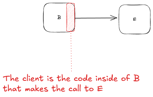
It could also refer to the code in the caller service that is responsible for making the request, typically packaged as a client library.
The fact that the meaning of these terms is ambiguous and context-dependent makes it harder to understand what someone is talking about when the term is used. While the person speaking knows exactly what sense of server, service or client they mean, the person hearing it does not.
The ambiguous meaning of these terms creates all sorts of problems, especially when communicating across different teams, where the meaning of a term used by the client team of a service may be different from the meaning of the term used by the owner of a service. I’m willing to bet that you, dear reader, have experienced this problem at some point in the past when reading an internal tech doc or trying to parse the meaning of a particular slack message.
As someone who is interested in incidents, I’m acutely aware of the problematic nature of ambiguous language during incidents, where communication and coordination play an enormous role in effective incident handling. But it’s not just an issue for incident handling. For example, Eric Evans advocates the use of ubiquitous language in software design. He pushes for consistent use of terms across different stakeholders to reduce misunderstandings.
In principle, we could all just decide to use more precise terminology. This would make it easier for listeners to understand the intent of speakers, and would reduce the likelihood of problems that stem from misunderstandings. At some level, this is the role that technical jargon plays. But client, server and serviceare technical jargon, and they’re still ambiguous. So, why don’t we just use even more precise language?
The problem is that expressing ourselves in unambiguous isn’t free: it costs the speaker additional effort to be more precise. As a trivial example, microservice is more precise than service, but it takes twice as long as to say, and it takes an additional five letters to write. Those extra syllables and letters are a cost to the speaker. And, all other things being equal, people prefer expending less effort than more effort. This is why we don’t like being on the receiving end of ambiguous language, because we have to put more effort into resolving the ambiguity through context clues.
The cost of precision to the speaker is clear in the world of computer programming. Traditional programming languages require an extremely high degree of precision on behalf of the coder. This sets a very high bar for being able to write programs. On the other hand, modern generative AI tools are able to take natural language inputs as specifications which are orders of magnitude less precise, and turn them into programs. These tools are able to process ambiguous inputs in ways that regular programming languages simply cannot. The cost in effort is much lower for the vibe programmer. (I will leave evaluation of the outcomes of vibe programming as an exercise for the reader).
Ultimately, the degree in precision in communication is a tradeoff: an increase in precision means less effort for the listener and less risk of misunderstanding, at a cost of more effort for the speaker. Because of this tradeoff, we shouldn’t expect the equilibrium point to be at maximal precision. Instead, it’s somewhere in the middle. Ideally, it would be where we minimize the total effort. Now, I’m not a cognitive scientist, but this is a theory that has been advanced by cognitive scientists. For example, see the paper The communicative function of ambiguity in language by Steven T. Piantadosi, Harry Tily, and Edward Gibson. I touched on the topic of ambiguity more generally in a previous post the high cost of low ambiguity.
We often ask “why are people doing X instead of the obviously superior Y“. This is an example of how we are likely missing the additional costs of choosing to do Y over X. Just because we don’t notice those costs doesn’t mean they aren’t there. It means we aren’t looking closely enough.
One of the topics I wrote about in my last post was about using formal methods to build a model of how our software behaves. In this post, I want to explore how the software we write itself contains models: models of how the world behaves.
The most obvious area is in our database schemas. These schemas enable us to digitally encode information about some aspect of the world that our software cares about. Heck, we even used to refer to this encoding of information into schemas as data models. Relational modeling is extremely flexible: in principle, we can represent just about any aspect of the world into it, if we put enough effort in. The challenge is that the world is messy, and this messiness significantly increases the effort required to build more complete models. Because we often don’t even recognize the degree of messiness the real world contains, we build over-simplified models that are too neat. This is how we end up with issues like the ones captured in Patrick McKenzie’s essay Falsehoods Programmers Believe About Names. There’s a whole book-length meditation on the messiness of real data and how it poses challenges for database modeling: Data and Reality by William Kent, which is highly recommended by Hillel Wayne, in his post Why You Should Read “Data and Reality”.
The problem of missing the messiness of the real world is not at all unique to software engineers. For example, see Christopher Alexander’s A City Is Not a Tree for a critique of urban planners’ overly simplified view of human interactions in urban environments. For a more expansive lament, check out James C. Scott’s excellent book Seeing Like a State. But, since I’m a software engineer and not an urban planner or a civil servant, I’m going to stick to the software side of things here.
Models in the back, models in the front
In particularly, my own software background is in the back-end/platform/infrastructure space. In this space, the software we write frequently implement control systems. It’s no coincidence that both cybernetics and kubernetes derived their names from the same ancient Greek word: κυβερνήτης. Every control system must contain within it a model of the system that it controls. Or, as Roger C. Conant and W. Ross Ashby put it, every good regulator of a system must be a model of that system.
Things get even more complex on the front-end side of the software world. This world must bridge the software world with the human world. In the context of Richard Cook’s framing in Above the Line, Below the Line, the front-end is the line that bridges the two world. As a consequence, the front-end’s responsibility is to expose a model of the software’s internal state to the user. This means that the front-end also has an implicit model of the users themselves. In the paper Cognitive Systems Engineering: New wine in new bottles, Erik Hollnagel and David Woods referred to this model as the image of the operator.
The dangers of the wrongness of models
There’s an oft-repeated quote by the statistician George E.P. Box: “All models are wrong but some are useful”. It’s a true statement, but one that focuses only on the upside of wrong models, the fact that some of them are useful. There’s also a downside to the fact that all models are wrong: the wrongness of these models can have drastic consequences.
And, while It’s a true statement, but what it fails to hint at how bad the consequences can be when a model is wrong. One of my favorite examples involves the 2008 financial crisis, as detailed by the journalist Felix Salmon’s 2009 Wired Magazine article Recipe for Disaster: The Formula that Killed Wall Street. The article described how Wall Street quants used a mathematical model known as the Gaussian copula function to estimate risk. It was a useful model that ultimately led to disaster.
Here’s A ripped-from-the-headlines example of image of the operator model error, how the U.S. national security advisor Mike Waltz accidentally saved the phone number of Jeffrey Goldberg, editor of the Atlantic magazine, to the contact information of White House spokesman Brian Hughes. The source is the recent Guardian story How the Atlantic’s Jeffrey Goldberg got added to the White House Signal group chat:
According to three people briefed on the internal investigation, Goldberg had emailed the campaign about a story that criticized Trump for his attitude towards wounded service members. To push back against the story, the campaign enlisted the help of Waltz, their national security surrogate.
Goldberg’s email was forwarded to then Trump spokesperson Brian Hughes, who then copied and pasted the content of the email – including the signature block with Goldberg’s phone number – into a text message that he sent to Waltz, so that he could be briefed on the forthcoming story.
Waltz did not ultimately call Goldberg, the people said, but in an extraordinary twist, inadvertently ended up saving Goldberg’s number in his iPhone – under the contact card for Hughes, now the spokesperson for the national security council.
…
According to the White House, the number was erroneously saved during a “contact suggestion update” by Waltz’s iPhone, which one person described as the function where an iPhone algorithm adds a previously unknown number to an existing contact that it detects may be related.
The software assumed that, when you receive a text from someone with a phone number and email address, that the phone number and email address belong to the sender. This is a model of the user that turned out to be very, very wrong.
Nobody expects model error
Software incidents involve model errors in one way or another, whether it’s an incorrect model of the system being controlled, an incorrect image of the operator, or a combination of the two.
And, yet, despite us all intoning “all models are wrong, some models are useful”, we don’t internalize that our systems our built on top of imperfect models. This is one of the ironies of AI: we are now all aware of the risks associated with model error with LLMs. We’ve even come up with a separate term for it: hallucinations. But traditional software is just as vulnerable to model error as LLMs are, because our software is always built on top of models that are guaranteed to be incomplete.
You’re probably familiar with the term black swan, popularized by the acerbic public intellectual Nassim Nicholas Taleb. While his first book, Fooled by Randomness, was a success, it was the publication of The Black Swan that made Taleb a household name, and introduced the public to the concept of black swans. While the term black swan was novel, the idea it referred to was not. Back in the 1980s, the researcher Zvi Lanir used a different term: fundamental surprise. Here’s an excerpt of a Richard Cook lecture on the 1999 Tokaimura nuclear accident where he talks about this sort of surprise (skip to the 45 minute mark).
And this Tokaimura accident was an impossible accident.
There’s an old joke about the creator of the first English American dictionary, Noah Webster … coming home to his house and finding his wife in bed with another man. And she says to him, as he walks in the door, she says, “You’ve surprised me”. And he says, “Madam, you have astonished me”.
The difference was that she of course knew what was going on, and so she could be surprised by him. But he was astonished. He had never considered this as a possibility.
And the Tokaimura was an astonishment or what some, what Zev Lanir and others have called a fundamental surprise which means a surprise that is fundamental in the sense that until you actually see it, you cannot believe that it is possible. It’s one of those “I can’t believe this has happened”. Not, “Oh, I always knew this was a possibility and I’ve never seen it before” like your first case of malignant hyperthermia, if you’re a an anesthesiologist or something like that. It’s where you see something that you just didn’t believe was possible. Some people would call it the Black Swan.
Black swans, astonishment, fundamental surprise, these are all synonyms for model error.
And these sorts of surprises are going to keep happening to us, because our models are always wrong. The question is: in the wake of the next incident, will we learn to recognize that fundamental surprises will keep happening to us in the future? Or will we simply patch up the exposed problems in our existing models and move on?