One of the criticisms leveled at resilience engineering is that the insights that the field generates aren’t actionable: “OK, let’s say you’re right, that complex systems are never perfectly understood, they’re always changing, they generate unexpected interactions, and that these properties explain why incidents happen. That doesn’t tell me what I should do about it!”
And it’s true; I can talk generally about the value of improving expertise so that we’re better able to handle incidents. But I can’t take the model of incidents that I’ve built based on my knowledge of resilience engineering and turn that into a specific software project that you can build and deploy that will eliminate a class of incidents.
But even if these insights aren’t actionable, that they don’t tell us about a single thing we can do or build to help improve reliability, my claim here is that these insights still have value. That’s because we as humans need models to make sense of the world, and if we don’t use good-but-not-actionable models, we can end up with actionable-but-not-good models. Or, as the statistics professor Andrew Gelman put it in his post The social sciences are useless. So why do we study them? Here’s a good reason back in 2021:
The baseball analyst Bill James once said that the alternative to good statistics is not no statistics, it’s bad statistics. Similarly, the alternative to good social science is not no social science, it’s bad social science.
The reason we do social science is because bad social science is being promulgated 24/7, all year long, all over the world. And bad social science can do damage.
Because we humans need models to make sense of the world, incidents models are inevitable. A good-but-not-actionable incident model will feel unsatisfying to people who are looking to leverage these models to take clear action. And it’s all too easy to build not-good-but-actionable models of how incidents happen. Just pick something that you can measure and that you theoretically have control over. The most common example of such a model is the one I’ll call “incidents happen because people don’t follow the processes that they are supposed to.” It’s easy to call out process violations in incident writeups, and it’s easy to define interventions to more strictly enforce processes, such as through automation.
In other words, good-but-not-actionable models protect us from the actionable-but-not-good models. They serve as a kind of vaccine, inoculating us from the neat, plausible, and wrong solutions that H.L. Mencken warned us about.
If you work in software, and I say the word server to you, which do you think I mean?
Software that responds to requests (e.g., http server)
A physical piece of hardware (e.g., a box that sits in a rack in a data center)
A virtual machine (e.g., an EC2 instance)
The answer, of course, is it depends on the context. The term server could mean any of those things. The term is ambiguous; it’s overloaded to mean different things in different contexts.
Another example of an overloaded term is service. From the end user’s perspective, the service is the system they interact with:
From the end user’s perspective, there is a single service
But if we zoom in on that box labeled service, it might be implemented by a collection of software components, where each component is also referred to as a service. This is sometimes referred to as a service-oriented architecture or a microservice architecture
A single “service” may be implemented by multiple “services”. What does “service” mean here?
Amusingly, when I worked at Netflix, people referred to microservices as “services”, but people also referred to all of Netflix as “the service”. For example, instead of saying, “What are you currently watching on Netflix?”, a person would say, “What are you currently watching on the service?”
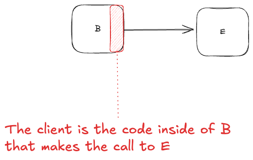
Yet another example is the term “client”. This could refer to the device that the end-user is using (e.g., web browser, mobile app):
Or it could refer to the caller service in a microservice architecture:
It could also refer to the code in the caller service that is responsible for making the request, typically packaged as a client library.
The fact that the meaning of these terms is ambiguous and context-dependent makes it harder to understand what someone is talking about when the term is used. While the person speaking knows exactly what sense of server, service or client they mean, the person hearing it does not.
The ambiguous meaning of these terms creates all sorts of problems, especially when communicating across different teams, where the meaning of a term used by the client team of a service may be different from the meaning of the term used by the owner of a service. I’m willing to bet that you, dear reader, have experienced this problem at some point in the past when reading an internal tech doc or trying to parse the meaning of a particular slack message.
As someone who is interested in incidents, I’m acutely aware of the problematic nature of ambiguous language during incidents, where communication and coordination play an enormous role in effective incident handling. But it’s not just an issue for incident handling. For example, Eric Evans advocates the use of ubiquitous language in software design. He pushes for consistent use of terms across different stakeholders to reduce misunderstandings.
In principle, we could all just decide to use more precise terminology. This would make it easier for listeners to understand the intent of speakers, and would reduce the likelihood of problems that stem from misunderstandings. At some level, this is the role that technical jargon plays. But client, server and serviceare technical jargon, and they’re still ambiguous. So, why don’t we just use even more precise language?
The problem is that expressing ourselves in unambiguous isn’t free: it costs the speaker additional effort to be more precise. As a trivial example, microservice is more precise than service, but it takes twice as long as to say, and it takes an additional five letters to write. Those extra syllables and letters are a cost to the speaker. And, all other things being equal, people prefer expending less effort than more effort. This is why we don’t like being on the receiving end of ambiguous language, because we have to put more effort into resolving the ambiguity through context clues.
The cost of precision to the speaker is clear in the world of computer programming. Traditional programming languages require an extremely high degree of precision on behalf of the coder. This sets a very high bar for being able to write programs. On the other hand, modern generative AI tools are able to take natural language inputs as specifications which are orders of magnitude less precise, and turn them into programs. These tools are able to process ambiguous inputs in ways that regular programming languages simply cannot. The cost in effort is much lower for the vibe programmer. (I will leave evaluation of the outcomes of vibe programming as an exercise for the reader).
Ultimately, the degree in precision in communication is a tradeoff: an increase in precision means less effort for the listener and less risk of misunderstanding, at a cost of more effort for the speaker. Because of this tradeoff, we shouldn’t expect the equilibrium point to be at maximal precision. Instead, it’s somewhere in the middle. Ideally, it would be where we minimize the total effort. Now, I’m not a cognitive scientist, but this is a theory that has been advanced by cognitive scientists. For example, see the paper The communicative function of ambiguity in language by Steven T. Piantadosi, Harry Tily, and Edward Gibson. I touched on the topic of ambiguity more generally in a previous post the high cost of low ambiguity.
We often ask “why are people doing X instead of the obviously superior Y“. This is an example of how we are likely missing the additional costs of choosing to do Y over X. Just because we don’t notice those costs doesn’t mean they aren’t there. It means we aren’t looking closely enough.
One of the topics I wrote about in my last post was about using formal methods to build a model of how our software behaves. In this post, I want to explore how the software we write itself contains models: models of how the world behaves.
The most obvious area is in our database schemas. These schemas enable us to digitally encode information about some aspect of the world that our software cares about. Heck, we even used to refer to this encoding of information into schemas as data models. Relational modeling is extremely flexible: in principle, we can represent just about any aspect of the world into it, if we put enough effort in. The challenge is that the world is messy, and this messiness significantly increases the effort required to build more complete models. Because we often don’t even recognize the degree of messiness the real world contains, we build over-simplified models that are too neat. This is how we end up with issues like the ones captured in Patrick McKenzie’s essay Falsehoods Programmers Believe About Names. There’s a whole book-length meditation on the messiness of real data and how it poses challenges for database modeling: Data and Reality by William Kent, which is highly recommended by Hillel Wayne, in his post Why You Should Read “Data and Reality”.
The problem of missing the messiness of the real world is not at all unique to software engineers. For example, see Christopher Alexander’s A City Is Not a Tree for a critique of urban planners’ overly simplified view of human interactions in urban environments. For a more expansive lament, check out James C. Scott’s excellent book Seeing Like a State. But, since I’m a software engineer and not an urban planner or a civil servant, I’m going to stick to the software side of things here.
Models in the back, models in the front
In particularly, my own software background is in the back-end/platform/infrastructure space. In this space, the software we write frequently implement control systems. It’s no coincidence that both cybernetics and kubernetes derived their names from the same ancient Greek word: κυβερνήτης. Every control system must contain within it a model of the system that it controls. Or, as Roger C. Conant and W. Ross Ashby put it, every good regulator of a system must be a model of that system.
Things get even more complex on the front-end side of the software world. This world must bridge the software world with the human world. In the context of Richard Cook’s framing in Above the Line, Below the Line, the front-end is the line that bridges the two world. As a consequence, the front-end’s responsibility is to expose a model of the software’s internal state to the user. This means that the front-end also has an implicit model of the users themselves. In the paper Cognitive Systems Engineering: New wine in new bottles, Erik Hollnagel and David Woods referred to this model as the image of the operator.
The dangers of the wrongness of models
There’s an oft-repeated quote by the statistician George E.P. Box: “All models are wrong but some are useful”. It’s a true statement, but one that focuses only on the upside of wrong models, the fact that some of them are useful. There’s also a downside to the fact that all models are wrong: the wrongness of these models can have drastic consequences.
And, while It’s a true statement, but what it fails to hint at how bad the consequences can be when a model is wrong. One of my favorite examples involves the 2008 financial crisis, as detailed by the journalist Felix Salmon’s 2009 Wired Magazine article Recipe for Disaster: The Formula that Killed Wall Street. The article described how Wall Street quants used a mathematical model known as the Gaussian copula function to estimate risk. It was a useful model that ultimately led to disaster.
Here’s A ripped-from-the-headlines example of image of the operator model error, how the U.S. national security advisor Mike Waltz accidentally saved the phone number of Jeffrey Goldberg, editor of the Atlantic magazine, to the contact information of White House spokesman Brian Hughes. The source is the recent Guardian story How the Atlantic’s Jeffrey Goldberg got added to the White House Signal group chat:
According to three people briefed on the internal investigation, Goldberg had emailed the campaign about a story that criticized Trump for his attitude towards wounded service members. To push back against the story, the campaign enlisted the help of Waltz, their national security surrogate.
Goldberg’s email was forwarded to then Trump spokesperson Brian Hughes, who then copied and pasted the content of the email – including the signature block with Goldberg’s phone number – into a text message that he sent to Waltz, so that he could be briefed on the forthcoming story.
Waltz did not ultimately call Goldberg, the people said, but in an extraordinary twist, inadvertently ended up saving Goldberg’s number in his iPhone – under the contact card for Hughes, now the spokesperson for the national security council.
…
According to the White House, the number was erroneously saved during a “contact suggestion update” by Waltz’s iPhone, which one person described as the function where an iPhone algorithm adds a previously unknown number to an existing contact that it detects may be related.
The software assumed that, when you receive a text from someone with a phone number and email address, that the phone number and email address belong to the sender. This is a model of the user that turned out to be very, very wrong.
Nobody expects model error
Software incidents involve model errors in one way or another, whether it’s an incorrect model of the system being controlled, an incorrect image of the operator, or a combination of the two.
And, yet, despite us all intoning “all models are wrong, some models are useful”, we don’t internalize that our systems our built on top of imperfect models. This is one of the ironies of AI: we are now all aware of the risks associated with model error with LLMs. We’ve even come up with a separate term for it: hallucinations. But traditional software is just as vulnerable to model error as LLMs are, because our software is always built on top of models that are guaranteed to be incomplete.
You’re probably familiar with the term black swan, popularized by the acerbic public intellectual Nassim Nicholas Taleb. While his first book, Fooled by Randomness, was a success, it was the publication of The Black Swan that made Taleb a household name, and introduced the public to the concept of black swans. While the term black swan was novel, the idea it referred to was not. Back in the 1980s, the researcher Zvi Lanir used a different term: fundamental surprise. Here’s an excerpt of a Richard Cook lecture on the 1999 Tokaimura nuclear accident where he talks about this sort of surprise (skip to the 45 minute mark).
And this Tokaimura accident was an impossible accident.
There’s an old joke about the creator of the first English American dictionary, Noah Webster … coming home to his house and finding his wife in bed with another man. And she says to him, as he walks in the door, she says, “You’ve surprised me”. And he says, “Madam, you have astonished me”.
The difference was that she of course knew what was going on, and so she could be surprised by him. But he was astonished. He had never considered this as a possibility.
And the Tokaimura was an astonishment or what some, what Zev Lanir and others have called a fundamental surprise which means a surprise that is fundamental in the sense that until you actually see it, you cannot believe that it is possible. It’s one of those “I can’t believe this has happened”. Not, “Oh, I always knew this was a possibility and I’ve never seen it before” like your first case of malignant hyperthermia, if you’re a an anesthesiologist or something like that. It’s where you see something that you just didn’t believe was possible. Some people would call it the Black Swan.
Black swans, astonishment, fundamental surprise, these are all synonyms for model error.
And these sorts of surprises are going to keep happening to us, because our models are always wrong. The question is: in the wake of the next incident, will we learn to recognize that fundamental surprises will keep happening to us in the future? Or will we simply patch up the exposed problems in our existing models and move on?
If you’re a regular reader of this blog, you’ll have noticed that I tend to write about two topics in particular:
Resilience engineering
Formal methods
I haven’t found many people who share both of these interests.
At one level, this isn’t surprising. Formal methods people tend to have an analytic outlook, and resilience engineering people tend to have a synthetic outlook. You can see the clear distinction between these two perspectives in the transcript of Leslie Lamport’s talk entitled The Future of Computing: Logic or Biology. Lamport is clearly on the side of the logic, so much so that he ridicules the very idea of taking a biological perspective on software systems. By contrast, resilience engineering types actively look to biology for inspiration on understanding resilience in complex adaptive systems. A great example of this is the late Richard Cook’s talk on The Resilience of Bone.
And yet, the two fields both have something in common: they both recognize the value of creating explicit models of aspects of systems that are not typically modeled.
You use formal methods to build a model of some aspect of your software system, in order to help you reason about its behavior. A formal model of a software system is a partial one, typically only a very small part of the system. That’s because it takes effort to build and validate these models: the larger the model, the more effort it takes. We typically focus our models on a part of the system that humans aren’t particularly good at reasoning about unaided, such as concurrent or distributed algorithms.
The act of creating and explicit model and observing its behavior with a model checker gives you a new perspective on the system being modeled, because the explicit modeling forces you to think about aspects that you likely wouldn’t have considered. You won’t say “I never imagined X could happen” when building this type of formal model, because it forces you to explicitly think about what would happen in situations that you can gloss over when writing a program in a traditional programming language. While the scope of a formal model is small, you have to exhaustively specify the thing within the scope you’ve defined: there’s no place to hide.
Resilience engineering is also concerned with explicit models, in two different ways. In one way, resilience engineering stresses the inherent limits of models for reasoning about complex systems (c.f., itsonlyamodel.com). Every model is incomplete in potentially dangerous ways, and every incident can be seen through the lens of model error: some model that we had about the behavior of the system turned out to be incorrect in a dangerous way.
But beyond the limits of models, what I find fascinating about resilience engineering is the emphasis on explicitly modeling aspects of the system that are frequently ignored by traditional analytic perspectives. Two kinds of models that come up frequently in resilience engineering are mental models and models of work.
A resilience engineering perspective on an incident will look to make explicit aspects of the practitioners’ mental models, both in the events that led up to that incident, and in the response to the incident. When we ask “How did the decision make sense at the time?“, we’re trying to build a deeper understanding of someone else’s state of mind. We’re explicitly trying to build a descriptive model of how people made decisions, based on what information they had access to, their beliefs about the world, and the constraints that they were under. This is a meta sort of model, a model of a mental model, because we’re trying to reason about how somebody else reasoned about events that occurred in the past.
A resilience engineering perspective on incidents will also try to build an explicit model of how work happens in an organization. You’ll often heard the short-hand phrase work-as-imagined vs work-as-done to get at this modeling, where it’s the work-as-done that is the model that we’re after. The resilience engineering perspective asserts that the documented processes of how work is supposed to happen is not an accurate model of how work actually happens, and that the deviation between the two is generally successful, which is why it persists. From resilience engineering types, you’ll hear questions in incident reviews that try to elicit some more details about how the work really happens.
Like in formal methods, resilience engineering models only get at a small part of the overall system. There’s no way we can build complete models of people’s mental models, or generate complete descriptions of how they do their work. But that’s ok. Because, like the models in formal methods, the goal is not completeness, but insight. Whether we’re building a formal model of a software system, or participating in a post-incident review meeting, we’re trying to get the maximum amount of insight for the modeling effort that we put in.
Brian Marick posted on Mastodon the other day about resilience in the context of governmental efficiency. Reading that inspired me to write about some more general observations about resilience.
Now, people use the term resiliencein different ways. I’m using resilience here in the following sense: how well a system is able to cope when it is pushed beyond its limits. Or, to borrow a term from safety researcher David Woods, when the system is pushed outside of its competence envelope. The technical term for this sense of the word resilience is graceful extensibility, which also comes from Woods. This term is a marriage of two other terms: graceful degradation, and software extensibility.
The term graceful degradation refers to the behavior of a system which, when it experiences partial failures, can still provide some functionality, even though it’s at a reduced fidelity. For example, for a web app, this might mean that some particular features are unavailable, or that some percentage of users are not able to access the site. Contrast this with a system that just returns 500 errors for everyone whenever something goes wrong.
We talk about extensible software systems as ones that have been designed to make it easy to add new features in the future that were not originally anticipated. A simple example of software extensibility is the ability for old code to callnew code, with dynamic binding being one way to accomplish this.
Now, putting those two concepts together, if a system encounters some sort of shock that it can’t handle, and the system has the ability to extend itself so that it can now handle the shock, and it can make these changes to itself quickly enough that it minimizes the harms resulting from the shock, then we say the system exhibits graceful extensibility. And if it can keep extending itself each time it encounters a novel shock, then we say that the system exhibits sustained adaptability.
The rest of this post is about the preconditions for resilience. I’m going to talk about resilience in the context of dealing with incidents. Note that all of the topics described below come from the resilience engineering literature, although I may not always use the same terminology.
As we discovered with Covid, efficiency is inversely correlated with resilience.
Here’s a question you can ask anyone who works in the compute infrastructure space: “How hot do you run your servers?” Or, even more meaningfully, “How much headroom do your servers have?”
Running your servers “hotter” means running at a higher CPU utilization. This means that you pack more load on fewer servers, which is more efficient. The problem is that the load is variable, which means that the hotter you run the servers, the more likely your server will get overloaded if there is a spike in utilization. An overloaded server can lead to an incident, and incidents are expensive! Running your servers at maximum utilization is running with zero headroom. We deliberately run our servers with some headroom to be able to handle variation in load.
We also see the idea of spare resources in what we call failover scenarios, where there’s a failure in one resource so we switch to using a different resource, such as failing over a database from primary to secondary, or even failing out of a geographical region.
The idea of spare resources is more general than hardware. It applies to people as well. The equivalent of headroom for humans is what Tom DeMarco refers to as slack. The more loaded humans are, the less well positioned they are to handle spikes in their workload. Stuff falls through the cracks when you’ve got too much load, and some of that stuff contributes to incidents. We can also even keep people in reserve for dealing with shocks, such as when an organization staffs a dedicated incident management team.
A common term that the safety people use for spare resources is capacity. I really like the way Todd Conklin put it on his Pre-Accident Investigation Podcast: “You don’t manage risk. You manage the capacity to absorb risk.” Another way he put it is “Accidents manage you, so what you really manage is the capacity for the organization to fail safely.”
Flexibility
Here’s a rough and ready definition of an incident: the system has gotten itself into a bad state, and it’s not going to return to a good state unless somebody does something about it.
Now, by this definition, for the system to become healthy again something about how the system works has to change. This means we need to change the way we do things. The easier it is to make changes to the system, the easier it will be to resolve the incident.
We can think of two different senses of changing the work of the system: the human side and the the software side.
Humans in a system are constrained by a set of rules that exist to reduce risk. We don’t let people YOLO code from their laptops into production, because of a number of risks that would expose us to. But incidents create scenarios where the risks associated with breaking these rules are lower than the risks associated with prolonging the incident. As a consequence, people in the system need the flexibility to be able to break the standard rules of work during an incident. One way to do this is to grant incident responders autonomy, let them make judgments about when they are able to break the rules that govern normal work, in scenarios where breaking the rule is less risky than following it.
Things look different on the software side, where all of the rules are mechanically enforced. For flexibility in software, we need to build into the software functionality in advance that will let us change the way the system behaves. My friend Aaron Blohowiak uses the term Jefferies tubesfrom Star Trek to describe features that support making operational changes to a system. These were service crawlways that made it easier for engineers to do work on the ship.
A simple example of this type of operational flexibility is putting in feature flags that can be toggled dynamically in order to change system behavior. At the other extreme is the ability to bring up a REPL on a production system in order to make changes. I’ve seen this multiple times in my career, including watching someone use the rails console command of a Ruby on Rails app to resolve an issue.
The technical term in resilience engineering for systems that possess this type of flexibility is adaptive capacity: the system has built up the ability to be able to dynamically reconfigure itself, to adapt, in order to meet novel challenges. This is where the name Adaptive Capacity Labs comes from.
Expertise
In general, organizations push against flexibility because it brings risk. In the case where I saw someone bring up a Ruby on Rails console, I was simultaneously impressed and terrified: that’s so dangerous!
Because flexibility carries risk, we need to rely on judgment as to whether the risk of leveraging the flexibility outweighs the risk of not using the flexibility to mitigate the incident. Granting people the autonomy to make those judgment calls isn’t enough: the people making the calls need to be able to make good judgment calls. And for that, you need expertise.
The people making these calls are having to make decisions balancing competing risks while under uncertainty and time pressure. In addition, how fluent they are with the tools is a key factor. I would never trust a novice with access to a REPL in production. But an expert? By definition, they know what they’re doing.
Diversity
Incidents in complex systems involve interactions between multiple parts of the system, and there’s no one person in your organization who understands the whole thing. To be able to effectively know what to do during an incident, you need to bring in different people who understand different parts of the system in order to help figure out what happens. You need diversity in your responders, people with different perspective on the problem at hand.
You also want diversity in diagnostic and mitigation strategy. Some people might think about recent changes, others might think about traffic pattern changes, others might dive into the codebase looking for clues, and yet others might look to see if there’s another problem going on right now that seems to be related. In addition, it’s often not obvious what the best course of action is to mitigate an incident. Responders often pursue multiple courses of action in parallel, hoping that at least one of them will bring the system healthy again. A diversity of perspectives can help generate more potential interventions, reducing the time to resolve.
Coordination
Having a group of experts with a diverse set of perspectives by itself isn’t enough to deal with an incident. For a system to be resilient, the people within the system need to be able to coordinate, to work together effectively.
If you’ve ever dealt with a complex incident, you know how challenging coordination can be. Things get even hairier in our distributed world. Whether you’re physically located with all of the responders, you’re on a Zoom call (a bridge, as we still say), you’re messaging over Slack, or some hybrid combination of all three, each type of communication channel has its benefits and drawbacks.
The next time you observe an incident, or you reflect on an incident where you were one of the responders, think back on to what extent these ingredients were present or absent. Were you able to leverage spare resources, or did you suffer from not being to? Were there operational changes that people wanted to be able to make during the incident, and were they actually able to make them? Were the responders experienced with the sub-systems they were dealing with, and how did that shape their responses? Did different people come up with different hypotheses and strategies? What is it clear to you what the different responders were doing during the incident? These issues are easy to miss if you’re not looking for them. But, once you internalize them, you’ll never be able to unsee them.
The amount of attention an incident gets is proportional to the severity of the incident: the greater the impact to the organization, the more attention that post-incident activities will get. It’s a natural response, because the greater the impact, the more unsettling it is to people: they worry very specifically about that incident recurring, and want to prevent that from happening again.
Here’s the problem: most of your incidents aren’t going to repeat incidents. Nobody wants an incident to recur, and so there’s a natural built-in mechanism for engineering teams to put in the effort to do preventative work. The real challenge is preventing and quickly mitigating novel future incidents, which is the overwhelming majority of your incidents.
And that brings us to near misses, those operational surprises that have no actual impact, but could have been a major incident if conditions were slightly different. Think of them as precursors to incidents. Or, if you are more poetically inclined, omens.
Because most of our incidents are novel, and because near misses are a source of insight about novel future incidents, if we are serious about wanting to improve reliability, we should be treating our near misses as first-class entities, the way we do with incidents. Yet, I’d wager that there are no tech companies out there today that would put the same level of effort into a near miss as they would to a real incident. I’d love to hear about a tech company that holds near miss reviews, but I haven’t heard any yet.
There are real challenges to treating near misses as first-class. We can generally afford to spend a lot of post-incident effort on each high-severity incident, because there generally aren’t that many of them. I’m quite confident that your org encounters many more near misses than it does high-severity incidents, and nobody has the cycles to put in the same level of effort for every near-miss as they do for every high severity incident. This means that we need to use judgment. We can’t use severity of impact to guide us here, because these near misses are, by definition, zero severity. We need to identify which near misses are worth examining further, and which ones to let go. It’s going to be a judgment call about how much we think we could potentially learn from looking further.
The other challenge is just surfacing these near misses. Because they are zero impact, it’s likely that only a handful of people in the organization are aware when a near miss happens. Treating near misses as first class events requires a cultural shift in an organization, where the people who are aware of them highlight the near miss as a potential source of insight for improving reliability. People have to see the value in sharing when these happens, it has to be rewarded or it won’t happen.
These near misses are happening in your organization right now. Some of them will eventually blossom into full-blown high-severity incidents. If you’re not looking for them, you won’t see them.
The California-based blogger Kevin Drum has a good post up today with the title Why don’t we do more prescribed burning? An explainer. There’s a lot of great detail in the post, but the bit that really jumped out at me was the history of the enormous forest fires that burned in Yellowstone National Park in 1988.
Norris Geyser Basin in Yellowstone National Park, August 20, 1988 By Jeff Henry – National Park Service archives, Public Domain
In 1988 the US Park Service allowed several lightning fires to burn in Yellowstone, eventually causing a conflagration that consumed over a million acres. Public fury was intense. In a post-mortem after the fire:
The team reaffirmed the fundamental importance of fire’s natural role but recommended that fire management plans be strengthened…. Until new fire management plans were prepared, the Secretaries suspended all prescribed natural fire programs in parks and wilderness areas.
This, in turn, made me think about the U.S. government’s effort to vaccinate the population against a potential swine flu epidemic in 1976, under the Gerald Ford administration.
Gerald Ford receiving swine flu vaccine By David Hume Kennerly – Gerald R. Ford Presidential Library: B1874-07A, Public Domain
The Swine Flu Program was marred by a series of logistical problems ranging from the production of the wrong vaccine strain to a confrontation over liability protection to a temporal connection of the vaccine and a cluster of deaths among an elderly population in Pittsburgh. The most damning charge against the vaccination program was that the shots were correlated with an increase in the number of patients diagnosed with an obscure neurological disease known as Guillain–Barré syndrome. The program was halted when the statistical increase was detected, but ultimately the New York Times labeled the program a “fiasco” because the feared pandemic never appeared.
Fortunately, swine flu didn’t become an epidemic, but it’s easy to imagine an alternative history where the epidemic materialized. In that scenario, the U.S. population would have suffered because the vaccination program was stopped. I don’t know how this experience shaped the minds of policymakers at the U.S. Centers for Disease Control (CDC), but I can certainly imagine the memories of the swine flu “fiasco” influencing of the calculus of how early to start pushing for a vaccine. After all, look what happened when we tried to head off a potential pandemic last time?
When a high-severity incident happens, its associated risks becomes salient: the incident looms large in our mind, and the fact that it just happened leads us to believe that the risk of a similar incident is very high. Suddenly, folks who normally extol the virtues of being data-driven are all too comfortable extrapolating from a single data point. But this tendency to fixate on a particular risk is dangerous, for the following two reasons:
We continually face a multitude of risks, not just a single one.
Risks trade off of each other.
We don’t deal in an individual risk but with a vast and ever-growing menu of risks. At best, when we focus on only risk, we pay the opportunity cost of neglecting the other ones. Attention is a precious resource, and focusing our attention on one particular risk means, necessarily, that we will neglect other risks.
But it’s even worse than that. In our effort to drive down a risk that just manifested as an incident, we end up increasing risk of a future incident. Fire suppression is a clear example of how an action taken to reduce risk can increase increase risk.
As Richard Cook noted, all practitioner actions are gambles. We don’t get to choose between “more safe” and “less safe”. The decisions we make always carry risk because of the uncertainties: we just can’t predict the future well enough to understand how our actions will reshape the risks. Remember that the next time people rush to address the risks exposed by the last major incident. Because the fact that an incident just happened does not improve your ability to predict the future, no matter how severe that incident was. All of those other risks are still out there, waiting to manifest as different incidents altogether. Your actions might even end up making those future incidents worse.
Today’s public incident writeup comes courtesy of Brendan Humphries, the CTO of Canva. Like somanyotherincidents that came before, this is another tale of saturation, where the failure mode involves overload. There’s a lot of great detail in Humpries’s write-up, and I recommend you read it directly in addition to this post.
What happened at Canva
Trigger: deploying a new version of a page
The trigger for this incident was Canva deploying a new version of their editor page. It’s notable that there was nothing wrong with this new version. The incident wasn’t triggered by a bug in the code in the new version, or even by some unexpected emergent behavior in the code of this version. No, while the incident was triggered by a deploy, the changes from the previous version are immaterial to this outage. Rather, it was the system behavior that emerged from clients downloading the new version that led to the outage. Specifically, it was clients downloading the new javascript files from the CDN that set the ball in motion.
A stale traffic rule
Canva uses Cloudflare as their CDN. Being a CDN, Cloudflare has datacenters all over the world., which are interconnected by a private backbone. Now, I’m not a networking person, but my basic understanding of private backbones is that CDNs lease fibre-optic lines from telecom companies and use these leased lines to ensure that they have dedicated network connectivity and bandwidth between their sites.
Unfortunately for Canva, there was a previously unknown issue on Cloudflare’s side: Cloudflare Wasn’t using their dedicated fibre-optic lines to route traffic between their Northern Virginia and Singapore datacenters. That traffic was instead, unintentionally, going over the public internet.
[A] stale rule in Cloudflare’s traffic management system [that] was sending user IPv6 traffic over public transit between Ashburn and Singapore instead of its default route over the private backbone.
Traffic between Northern Virginia (IAD) and Singapore (SIN) was incorrectly routed over the public network
The routes that this traffic took suffered from considerable packet loss. For Canva users in Asia, this meant that they experienced massive increases in latency when their web browsers attempted to fetch the javascript static assets from the CDN.
A stale rule like this is the kind of issue that the safety researcher James Reason calls a latent pathogen. It’s a problem that remains unnoticed until it emerges as a contributor to an incident.
High latency synchronizes the callers
Normally, an increase in errors would cause our canary system to abort a deployment. However, in this case, no errors were recorded because requests didn’t complete. As a result, over 270,000+ user requests for the JavaScript file waited on the same cache stream. This created a backlog of requests from users in Southeast Asia.
The first client attempts to fetch the new Javascript files from the CDN, but the files aren’t there yet, the CDN must fetch the files from the origin. Because of the added latency, this takes a long time.
During this time, other clients connect, and attempt to fetch the javascript from the CDN. But the CDN has not yet been populated with the files from the origin, that transfer is still in progress.
As Cloudflare notes in this blog post, when all subsequent clients request access to a file that is in the process of being populated in the cache, they must wait until the file has been cached before they can download the file. Except that Cloudflare has implemented functionality called Concurrent Streaming Acceleration which permits multiple clients to simultaneously download a file that is still in the process of being downloaded from the origin server.
The resulting behavior is that the CDN now behaves effectively as a barrier, with all of the clients slowly but simultaneously downloading the assets. With a traditional barrier, the processes who are waiting can proceed once all processes have entered in the barrier. This isn’t quite the same, as the clients who are waiting can all proceed once the CDN completes downloading the asset from the origin.
The transfer completes, the herd thunders
At 9:07 AM UTC, the asset fetch completed, and all 270,000+ pending requests were completed simultaneously.
20 minutes after Canva deployed the new Javascript assets to the origin server, the clients completed fetching them. The next action the clients take is to call Canva’s API service.
With the JavaScript file now accessible, client devices resumed loading the editor, including the previously blocked object panel. The object panel loaded simultaneously across all waiting devices, resulting in a thundering herd of 1.5 million requests per second to the API Gateway — 3x the typical peak load.
There’s one more issue that made this situation even worse: a known performance issue in the API gateway that was slated to be fixed.
A problematic call pattern to a library reduces service throughput
The API Gateways use an event loop model, where code running on event loop threads must not perform any blocking operations.
Two common threading models for request-response services are thread-per-request and async. For services that are I/O-bound (i.e., most of the time servicing each request is spent waiting for I/O operations to complete, typically networking operations), the async model has the potential to achieve better throughput. That’s because the concurrency of the thread-per-request model is limited by the number of operating-system threads. The async model services multiple requests per thread, and so it doesn’t suffer from the thread bottleneck. Canva’s API gateway implements the async model using the popular Netty library.
One of the drawbacks of the async model is the risk associated with the active thread getting blocked, because this can result in a significant performance penalty. The async model multiplexes multiple requests across an individual thread, and none of those requests can make progress when that thread is blocked. Programmers writing code in a service that uses the async model need to take care to minimize the number of blocking calls.
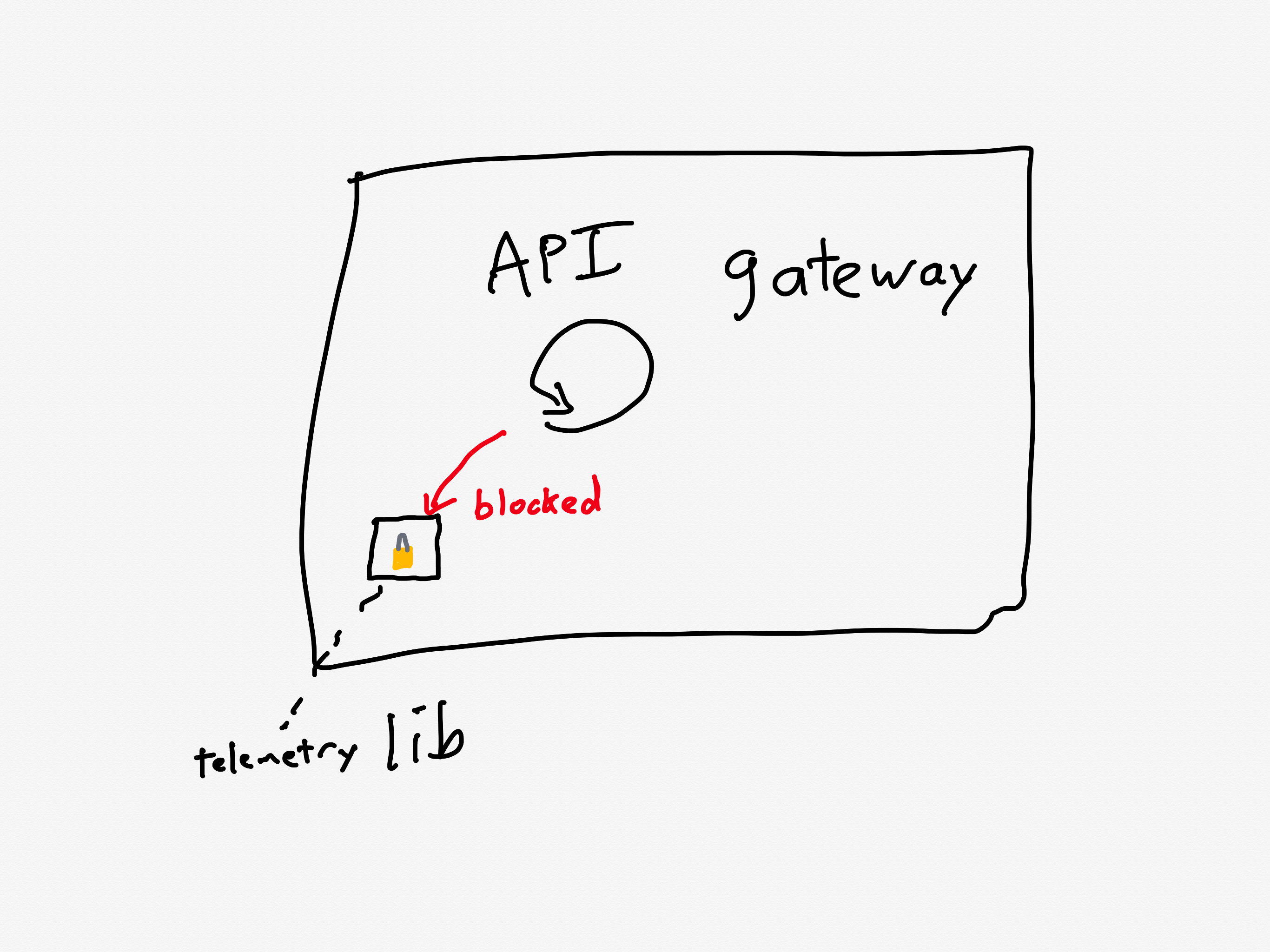
Prior to this incident, we’d made changes to our telemetry library code, inadvertently introducing a performance regression. The change caused certain metrics to be re-registered each time a new value was recorded. This re-registration occurred under a lock within a third-party library.
In Canva’s case, the API gateway logic was making calls to a third-party telemetry library. They were calling the library in such a way that it took a lock, which is a blocking call. This reduced the effective throughput that the API gateway could handle.
Calls to the library led to excessive thread locking
Although the issue had already been identified and a fix had entered our release process the day of the incident, we’d underestimated the impact of the bug and didn’t expedite deploying the fix. This meant it wasn’t deployed before the incident occurred.
Ironically, they were aware of this problematic call pattern, and they were planning on deploying a fix the day of the incident(!).
Canva is now in a situation where the API gateway is receiving much more traffic than it was provisioned to handle, is also suffering from a performance regression that reduces its ability to handle traffic even more.
Now let’s look at how the system behaved under these conditions.
The load balancer turns into an overload balancer
Because the API Gateway tasks were failing to handle the requests in a timely manner, the load balancers started opening new connections to the already overloaded tasks, further increasing memory pressure.
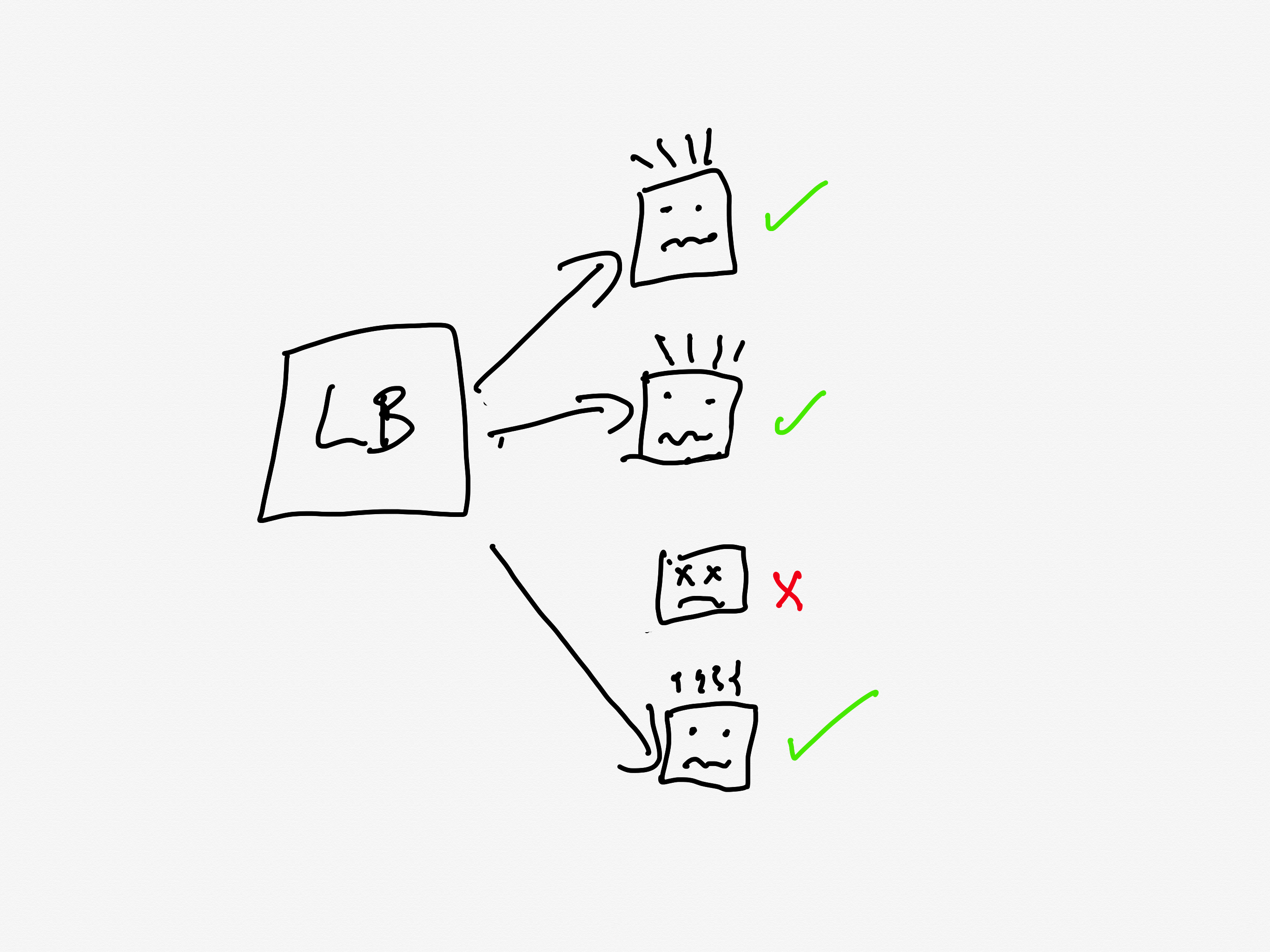
A load balancer sits in front of a service and distributes the incoming requests across the units of compute. Canva runs atop ECS, so the individual units are called tasks, and the group is called a cluster (you can think of these as being equivalent to pods and replicasets in Kubernetes-land).
The load balancer will only send requests to a task that is healthy. If a task is unhealthy, then it stops being considered as a candidate target destination for the load balancer. This yields good results if the overall cluster is provisioned to handle the load: the traffic gets redirected away from the unhealthy tasks and onto the healthy ones.
Load balancer only sells traffic to the healthy tasks
But now consider the scenario where all of the tasks are operating close to capacity. As tasks go unhealthy, the load balancer will redistribute the load to the remaining “healthy” tasks, which increases the likelihood those tasks gets pushed into an unhealthy state.
Redirecting traffic to the almost-overloaded healthy nodes will push them over
This is a classic example of a positive feedback loop: the more tasks go unhealthy, the more traffic the healthy nodes received, the more likely those tasks will go unhealthy as well.
Autoscaling can’t keep pace
So, now the system is saturated, and the load balancer is effectively making things worse. Instead of shedding load, it’s concentrating load on the tasks that aren’t overloaded yet.
Now, this is the cloud, and the cloud is elastic, and we have a wonderful automation system called the autoscaler that can help us in situations of overload by automating provisioning new capacity.
Only, there’s a problem here, and that’s that the autoscaler simply can’t scale up fast enough. And the reason it can’t scale up fast enough is because of another automation system that’s intended to help in times of overload: Linux’s OOM killer.
The growth of off-heap memory caused the Linux Out Of Memory Killer to terminate all of the running containers in the first 2 minutes, causing a cascading failure across all API Gateway tasks. This outpaced our autoscaling capability, ultimately leading to all requests to canva.com failing.
Operating systems need access to free memory in order to function properly. When all of the memory is consumed by running processes, the operating system runs into trouble. To guard against this, Linux has a feature called the OOM killer which will automatically terminate a process when the operating system is running too low on memory. This frees up memory, enabling the OS to keep functioning.
So, you have the autoscaler which is adding new tasks, and the OOM killer which is quickly destroying existing tasks that have become overloaded.
It’s notable that Humphries uses the term outpaced. This sort of scenario is a common failure mode in complex system failures, where the system gets into a state where it can’t keep up. This phenomenon is called decompensation. Here’s resilience engineering pioneer David Woods describing decompensation on John Willis’s Profound Podcast:
And lag is really saturation in time. That’s what we call decompensation, right? I can’t keep pace, right? Events are moving forward faster. Trouble is building and compounding faster than I, than the team, than the response system can decide on and deploy actions to affect. So I can’t keep pace. – David Woods
Adapting the system to bring it back up
At this point, the API gateway cluster is completely overwhelmed. From the timeline:
9:07 AM UTC – Network issue resolved, but the backlog of queued requests result in a spike of 1.5 million requests per second to the API gateway.
9:08 AM UTC – API Gateway tasks begin failing due to memory exhaustion, leading to a full collapse.
When your system is suffering from overload, there are basically two strategies:
increase the capacity
reduce the load
Wisely, the Canva engineers pursued both strategies in parallel.
Max capacity, but it still isn’t enough
Montgomery Scott, my nominee for patron saint of resilience engineering
We attempted to work around this issue by significantly increasing the desired task count manually. Unfortunately, it didn’t mitigate the issue of tasks being quickly terminated.
The engineers tried to increase capacity manually, but even with the manual scaling, the load was too much: the OOM killer was taking the tasks down too quickly for the system to get back to a healthy state.
Load shedding, human operator edition
The engineers had to improvise a load shedding solution in the moment. The approach they took was to block traffic the CDN layer, using Cloudflare.
At 9:29 AM UTC, we added a temporary Cloudflare firewall rule to block all traffic at the CDN. This prevented any traffic reaching the API Gateway, allowing new tasks to start up without being overwhelmed with incoming requests. We later redirected canva.com to our status page to make it clear to users that we were experiencing an incident.
It’s worth noting here that while Cloudflare contributed to this incident with the stale rule, the fact that they could dynamically configure Cloudflare firewall rules meant that Cloudflare also contributed to the mitigation of this incident.
Ramping the traffic back up
Here they turned off all of their traffic to give their system a chance to go back to healthy. But a healthy system under zero load behaves differently from a healthy system under typical load. If you just go back from zero to typical, there’s a risk that you push the system back into an unhealthy state. (One common problem is that autoscaling will have scaled down multiple services due when there’s no load).
Once the number of healthy API Gateway tasks stabilized to a level we were comfortable with, we incrementally restored traffic to canva.com. Starting with Australian users under strict rate limits, we gradually increased the traffic flow to ensure stability before scaling further.
The Canva engineers had the good judgment to ramp up the traffic incrementally rather than turn it back on all at once. They started restoring at 9:45 AM UTC, and were back to taking full traffic at 10:04 AM.
Some general observations
All functional requirements met
I always like to call out situations where, from a functional point of view, everything was actually working fine. In this case, even though there was a stale rule in the Cloudflare traffic management system, and there was a performance regression in the API gateway, everything was working correctly from a functional perspective: packets were still being routed between Singapore and Northern Virginia, and the API gateway was still returning the proper responses for individual requests before it got overloaded.
Rather, these two issues were both performance problems. Performance problems are much harder to spot, and the worst are the ones that you don’t notice until you’re under heavy load.
The irony is that, as an organization gets better at catching functional bugs before they hit production, more and more of the production incidents they face will be related to these more difficult-to-detect-early performance issues.
Automated systems made the problem worse
There were a number of automated systems in play whose behavior made this incident more difficult to deal with.
The Concurrent Streaming Acceleration functionality synchronized the requests from the clients. The OOM killer reduced the time it took for a task to be seen as unhealthy by the load balancer, and the load balancer in turn increased the rate at which tasks went unhealthy.
None of these systems were designed to handle this sort of situation, so they could not automatically change their behavior.
The human operators changed the way the system behaved
It was up to the incident responders to adapt the behavior of the system, to change the way it functioned in order to get it back to a healthy state. They were able to leverage an existing resource, Cloudflare’s firewall functionality, to accomplish this. Based on the description of the action items, I suspect they had never used Cloudflare’s firewall to do this type of load shedding before. But it worked! They successfully adapted the system behavior.
We’re building a detailed internal runbook to make sure we can granularly reroute, block, and then progressively scale up traffic. We’ll use this runbook to quickly mitigate any similar incidents in the future.
This is a classic example of resilience, of acting to reconfigure the behavior of your system when it enters a state that it wasn’t originally designed to handle.
As I’ve written about previously, Woods talks about the idea of a competence envelope. The competence envelope is sort of a conceptual space of the types of inputs that your system can handle. Incidents occur when your system is pushed to operate outside of its competence envelope, such as when it gets more load than it is provisioned to handle:
The competence envelope is a good way to think about the difference between robustness and resilience. You can think of robustness as describing the competence envelope itself: a more robust system may have a larger competence envelope, it is designed to handle a broader range of problems.
However, every system has a finite competence envelope. The difference between a resilient and a brittle system is how that system behaves when it is pushed just outside of its competence envelope.
Incidents happen when the system is pushed outside of its competence envelope
A resilient system can change the way it behaves when pushed outside of the competence envelope due to an incident in order to extend the competence envelope so that it can handle the incident. That’s why we say it has adaptive capacity. On the other hand, a brittle system is one that cannot adapt effectively when it exceeds its competence envelope. A system can be very robust, but also brittle: it may be able to handle a very wide range of problems, but when it faces a scenario it wasn’t designed to handle, it can fall over hard.
The sort of adaptation that resilience demands requires human operators: our automation simply doesn’t have a sophisticated enough model of the world to be able to handle situations like the one that Canva found itself in.
In general, action items after an incident focus on expanding the competence envelope: making changes to the system to handle the scenario that just happened. Improving adaptive capacity involves different kind of work than improving system robustness.
We need to build in the ability to reconfigure our systems in advance, without knowing exactly what sorts of changes we’ll need to make. The Canva engineers had some powerful operational knobs at their disposal through the Cloudflare firewall configuration. This allowed them to make changes. The more powerful and generic these sorts of dynamic configuration features are, the more room for maneuver we have. Of course, dynamic configuration is also dangerous, and is itself a contributor to incidents. Too often we focus solely on the dangers of such functionality in creating incidents, without seeing its ability to help us reconfigure the system to mitigate incidents.
Finally, these sorts of operator interfaces are of no use if the responders aren’t familiar with them. Ultimately, the more your responders know about the system, the better position they’ll be in to implement these adaptations. Changing an unhealthy system is dangerous: no matter how bad things are, you can always accidentally make things worse. The more knowledge about the system you can bring to bear during an incident, the better position you’ll be in to adaptive your system to extend that competence envelope.
OpenAI recently published a public writeup for an incident they had on December 11, and there are lots of good details in here! Here are some of my off-the-cuff observations:
Saturation
With thousands of nodes performing these operations simultaneously, the Kubernetes API servers became overwhelmed, taking down the Kubernetes control plane in most of our large clusters.
The term saturation describes the condition where a system has reached the limit of what it can handle. This is sometimes referred to as overload or resource exhaustion. In the OpenAI incident, it was the Kubernetes API servers saturated because they were receiving too much traffic. Once that happened, the API servers no longer functioned properly. As a consequence, their DNS-based service discovery mechanism ultimately failed.
Saturation is an extremely common failure mode in incidents, and here OpenAI provides us with yet another example. You can also read some previous posts about public incident writeups involving saturation: Cloudflare, Rogers, and Slack.
All tests pass
The change was tested in a staging cluster, where no issues were observed. The impact was specific to clusters exceeding a certain size, and our DNS cache on each node delayed visible failures long enough for the rollout to continue.
One reason why it’s difficult to prevent saturation-related incidents is because all of the software can be functionally correct, in the sense that it passes all of the functional tests and that the failure mode only rears its ugly head once the system is exposed to conditions that only occur in the production environment. Even canarying with production traffic can’t prevent problems that only occur under full load.
Our main reliability concern prior to deployment was resource consumption of the new telemetry service. Before deployment, we evaluated resource utilization metrics in all clusters (CPU/memory) to ensure that the deployment wouldn’t disrupt running services. While resource requests were tuned on a per cluster basis, no precautions were taken to assess Kubernetes API server load. This rollout process monitored service health but lacked sufficient cluster health monitoring protocols.
It’s worth noting that the engineers did validate the change in resource utilization on the clusters where the new telemetry configuration was deployed. The problem was an interaction: it increased load on the API servers, which brings us to the next point.
Complex, unexpected interactions
This was a confluence of multiple systems and processes failing simultaneously and interacting in unexpected ways.
When we look at system failures, we often look for problems in individual components. But in complex systems, identifying the complex, unexpectedinteractions can yield better insights into how failures happens. You don’t just want to look at the boxes, you also want to look at the arrows.
In short, the root cause was a new telemetry service configuration that unexpectedly generated massive Kubernetes API load across large clusters, overwhelming the control plane and breaking DNS-based service discovery.
“So, we rolled out the new telemetry service, and, yada yada yada, our services couldn’t call each other anymore.”
In this case, the surprising interaction was between a failure of the kubernetes API and the resulting failure of services running on top of kubernetes. Normally, if you have services that are running on top of kubernetes and your kubernetes API goes unhealthy, your services should still keep running normally, you just can’t make changes to your current deployment (e.g., deploy new code, change the number of pods). However, in this case, a failure in the kubernetes API (control plane) ultimately led to failures in the behavior of running services (data plane).
The coupling between the two? It was DNS.
DNS
In short, the root cause was a new telemetry service configuration that unexpectedly generated massive Kubernetes API load across large clusters, overwhelming the control plane and breaking DNS-based service discovery.
Impact of a change is spread out over time
DNS caching added a delay between making the change and when services started failing.
One of the things that makes DNS-related incidents difficult to deal with is the nature of DNS caching.
When the effect of a change is spread out over time, this can make it more difficult to diagnose what the breaking change was. This is especially true when the critical service that stopped working (in this case, service discovery) was not the thing that was changed (telemetry service deployment).
DNS caching made the issue far less visible until the rollouts had begun fleet-wide.
In this case, the effect was spread out over time because of the nature of DNS caching. But often we intentionally spread out a change over time because we want to reduce the blast radius if the change we are rolling out turns out to be a breaking change. This works well if we detect the problem during the rollout. However, this can also make it harder to detect the problem, because the error signal is smaller (by design!). And if we only detect the problem after the rollout is complete, it can be harder to correlate the change with the effect, because the change was smeared out over time.
Failure mode makes remediation more difficult
In order to make that fix, we needed to access the Kubernetes control plane – which we could not do due to the increased load to the Kubernetes API servers.
Sometimes the failure mode that breaks systems that production depends upon also breaks systems that operators depend on to do their work. I think James Mickens said it best when he wrote:
I HAVE NO TOOLS BECAUSE I’VE DESTROYED MY TOOLS WITH MY TOOLS
And as our engineers worked to figure out what was happening and why, they faced two large obstacles: first, it was not possible to access our data centers through our normal means because their networks were down, and second, the total loss of DNS broke many of the internal tools we’d normally use to investigate and resolve outages like this.
This type of problem often requires that operators improvise a solution in the moment. The OpenAI engineers pursued multiple strategies to get the system heathy again.
We identified the issue within minutes and immediately spun up multiple workstreams to explore different ways to bring our clusters back online quickly:
Scaling down cluster size: Reduced the aggregate Kubernetes API load.
Blocking network access to Kubernetes admin APIs: Prevented new expensive requests, giving the API servers time to recover.
Scaling up Kubernetes API servers: Increased available resources to handle pending requests, allowing us to apply the fix.
By pursuing all three in parallel, we eventually restored enough control to remove the offending service.
Their interventions were successful, but it’s easy to imagine scenarios where one of these interventions accidentally made things even worse. As Richard Cook noted: all practitioner actions are gambles. Incidents always involve uncertainty in the moment, and it’s easy to overlook this when we look back with perfect knowledge of how the events unfolded.
A change intended to improve reliability
As part of a push to improve reliability across the organization, we’ve been working to improve our cluster-wide observability tooling to strengthen visibility into the state of our systems. At 3:12 PM PST, we deployed a new telemetry service to collect detailed Kubernetes control plane metrics.
This is a great example of unexpected behavior of a subsystem whose primary purpose was to improve reliability. This is another data point for my conjecture on why reliable systems fail.
Well, who you gonna believe, me or your own eyes? – Chico Marx (dressed as Groucho), from Duck Soup:
In the ACM Queue article Above the Line, Below the Line, the late safety researcher Richard Cook (of How Complex Systems Fail fame) notes how that we software operators don’t interact directly with the system. Instead, we interact through representations. In particular, we view representations of internal state of the system, and we manipulate these representations in order to effect changes, to control the system. Cook used the term line of representation to describe the split between the world of the technical (software) system and the world of the people who work with the technical system. The people are above the line of representation, and the technical system is below the line.
Above the line of representation are the people, organizations, and processes that shape, direct, and restore the technical artifacts that lie below that line.People who work above the line routinely describe what is below the line using concrete, realistic language.
Yet, remarkably, nothing below the line can be seen or acted upon directly. The displays, keyboards, and mice that constitute the line of representation are the only tangible evidence that anything at all lies below the line. All understandings of what lies below the line are constructed in the sense proposed by Bruno Latour and Steve Woolgar. What we “know”—what we can know—about what lies below the line depends on inferences made from representations that appear on the screens and displays.
In short, we can never actually see or change the system directly, all of our interactions mediated through software interfaces.
René Magritte would have appreciated Cook’s article
In this post, I want to talk about how this fact can manifest as incidents, and that our solutions rarely consider this problem. Let’s start off, as we so often do in the safety world, with the Three Mile Island accident.
Three Mile Island and the indicator light
I assume the reader has some familiarity with the partial meltdown that occurred at the Three Mile Island nuclear plant back in 1979. As it happens, there’s a great series of lectures by Cook on accidents. The topic of his first lecture is about how Three Mile Island changed the way safety specialists thought about the nature of accidents.
Here I want to focus on just one aspect of this incident: a particular indicator light in the Three Mile Island control room. During this incident, there was a type of pressure relief valve called a pilot-operated relief valve (PORV) that was stuck open. However, the indicator light for the state of this valve was off, which the operators interpreted (incorrectly, alas) as the valve being closed. Here I’ll quote the wikipedia article:
A light on a control panel, installed after the PORV had stuck open during startup testing, came on when the PORV opened. When that light—labeled Light on – RC-RV2 open —went out, the operators believed that the valve was closed. In fact, the light when on only indicated that the PORV pilot valve’s solenoid was powered, not the actual status of the PORV. While the main relief valve was stuck open, the operators believed the unlighted lamp meant the valve was shut. As a result, they did not correctly diagnose the problem for several hours.
What I found notable was the article’s comment about lack of operator training to handle this specific scenario, a common trope in incident analysis.
The operators had not been trained to understand the ambiguous nature of the PORV indicator and to look for alternative confirmation that the main relief valve was closed. A downstream temperature indicator, the sensor for which was located in the tail pipe between the pilot-operated relief valve and the pressurizer relief tank, could have hinted at a stuck valve had operators noticed its higher-than-normal reading. It was not, however, part of the “safety grade” suite of indicators designed to be used after an incident, and personnel had not been trained to use it. Its location behind the seven-foot-high instrument panel also meant that it was effectively out of sight.
Now, consider what happens if the agent acting on these sensors is an automated control system instead of a human operator.
Sensors, automation, and accidents: cases from aviation
In the aviation world, we have a combination of automation and human operators (pilots) who work together in real-time. The assumption is that if something goes wrong with the automation, the human can quickly take over and deal with the problem. But automation can make things too difficult for a human to be able to compensate for, and automation can be particularly vulnerable to sensor problems, as we can see in the following accidents:
Bombardier Learjet 60 accident, 2008
On September 19, 2008, in Columbia, South Carolina, a Bombardier Learjet 60 overran the runway during a rejected takeoff. As a consequence, four people aboard the plane, including the captain and first officer, were killed. In this case, the sensor issues were due to damage to electronics in the wheel well area after underinflated tires on the landing gear exploded.
The pilots reversed thrust to slow down the plane. However, the tires on the plane were under-inflated, and they exploded. As a result of the tire explosion, sensors in the wheel well area of the plane were damaged.
The thrust reverse system relies on sensor data to determine whether reversing thrust is a safe operation. Because of the sensor damage, the system determined that it was not safe to reverse thrust, and instead increased forward thrust. From the NTSB report:
In this situation, the EECs would transition from the reverse thrust power schedule to the forward thrust power schedule during about a 2-second transition through idle power. During the entire sequence, the thrust reverser levers in the cockpit would remain in the reverse thrust idle position (as selected by the pilot) while the engines produced forward thrust. Because both the thrust reverser levers and the forward thrust levers share common RVDTs (one for the left engine and one for the right engine), the EECs, which receive TLA information from the RVDTs, would signal the engines to produce a level of forward thrust that generally corresponds with the level of reverse thrust commanded; that is, a pilot commanding full reverse thrust (for maximum deceleration of the airplane) would instead receive high levels of forward thrust (accelerating the airplane) according to the forward thrust power schedule
On June 1, 2009, Air France 447 crashed, killing all passengers and crew. The plane was an Airbus A330-200. In this accident, the sensor problem is believed to be caused by ice crystals that accumulated inside of pitot tube sensors, creating a blockage which lead to erroneous readings. Here’s a quote from an excellent Vanity Fair article on the crash:
Just after 11:10 P.M., as a result of the blockage, all three of the cockpit’s airspeed indications failed, dropping to impossibly low values. Also as a result of the blockage, the indications of altitude blipped down by an unimportant 360 feet. Neither pilot had time to notice these readings before the autopilot, reacting to the loss of valid airspeed data, disengaged from the control system and sounded the first of many alarms—an electronic “cavalry charge.” For similar reasons, the automatic throttles shifted modes, locking onto the current thrust, and the fly-by-wire control system, which needs airspeed data to function at full capacity, reconfigured itself from Normal Law into a reduced regime called Alternate Law, which eliminated stall protection and changed the nature of roll control so that in this one sense the A330 now handled like a conventional airplane. All of this was necessary, minimal, and a logical response by the machine.
This is what the safety researcher David Woods refers to as bumpy transfer of control, where the humans must suddenly and unexpectedly take over control of an automated system, which can lead to disastrous consequences.
Boeing 737 MAX 8 (2018, 2019)
On October 29, 2018, Lion Air Flight 610 crashed thirteen minutes after takeoff, killing everyone on board. Five months later, on March 10, 2019, Ethiopian Airlines Flight 302 crashed six minutes after takeoff, also killing everyone on board. Both planes were Boeing 737 MAX 8. In both cases, the sensor problem was related to the angle-of-attack (AOA) sensor.
The replacement AOA sensor that was installed on the accident aircraft had been mis-calibrated during an earlier repair. This mis-calibration was not detected during the repair.
Shortly after liftoff, the left Angle of Attack sensor recorded value became erroneous and the left stick shaker activated and remained active until near the end of the recording.
An automation subsystem in the 737 MAX called Maneuvering Characteristics Augmentation System (MCAS) automatically pushed the nose down in response to the AOA sensor data.
What should we take away from these?
Here I’ve given examples from aviation, but sensor-automation problems are not specific to that domain. Here are a few of my own takeaways.
We designers can’t assume sensor data will be correct
The kinds of safety automation subsystems we build in tech are pretty much always closed-loop control systems. When designing such systems in the tech world, how often have you heard someone ask, “what happens if there’s a problem with the sensor data that the system is reacting to?”
This goes back to the lineof representation problem: that no agent ever gets access to the true state of the system, it only gets access to some sort of representation. The irony here is that it doesn’t just apply to humans (above the line) making sense of signals, it also applies to technical system components (below the line!) making sense of signals from other technical components.
Designing a system that is safe in the face of sensor problems is hard
Again, from the NTSB report of the Learjet 60 crash:
Learjet engineering personnel indicated that the uncommanded stowage of the thrust reversers in the event of any system loss or malfunction is part of a fail-safe design that ensures that a system anomaly cannot result in a thrust reverser deployment in flight, which could adversely affect the airplane’s controllability. The design is intended to reduce the pilot’s emergency procedures workload and prevent potential mistakes that could exacerbate an abnormal situation.
The thrust reverser system behavior was designed by aerospace engineers to increase safety, and ended up making things worse! Good luck imagining all of these sorts of scenarios when you design your systems to increase safety.
Even humans struggle in the face of sensor problems
People are better equipped to handle sensor problems than automation, because we don’t seem to be able to build automation that can handle all of the possible kinds of sensor problems that we might throw at a problem.
But even for humans, sensor problems are difficult. While we’ll eventually figure out what’s going on, we’ll still struggle in the face of conflicting signals, as anyone who has responded to an incident can tell you. And in high-tempo situations, where we need to respond quickly enough or something terrible will happen (like in the Air France 447 case), we simply might not be able to respond quickly enough.
Instead of focusing on building the perfect fail-safe system to prevent this next time, I wish we’d spend more time thinking about, “how can we help the human figure out what the heck is happening when the input signals don’t seem to make sense”.